epi2024
epi2024.Rmd
set.seed(7865)
library(SMILE)
library(tidyverse)
#> Warning: package 'tidyverse' was built under R version 4.3.2
#> Warning: package 'ggplot2' was built under R version 4.3.2
#> Warning: package 'tibble' was built under R version 4.3.2
#> Warning: package 'tidyr' was built under R version 4.3.2
#> Warning: package 'readr' was built under R version 4.3.2
#> Warning: package 'purrr' was built under R version 4.3.2
#> Warning: package 'dplyr' was built under R version 4.3.2
#> Warning: package 'stringr' was built under R version 4.3.2
#> Warning: package 'forcats' was built under R version 4.3.2
#> Warning: package 'lubridate' was built under R version 4.3.2
#> ── Attaching core tidyverse packages ──────────────────────── tidyverse 2.0.0 ──
#> ✔ dplyr     1.1.4     ✔ readr     2.1.5
#> ✔ forcats   1.0.0     ✔ stringr   1.5.1
#> ✔ ggplot2   3.5.0     ✔ tibble    3.2.1
#> ✔ lubridate 1.9.3     ✔ tidyr     1.3.1
#> ✔ purrr     1.0.2
#> ── Conflicts ────────────────────────────────────────── tidyverse_conflicts() ──
#> ✖ dplyr::filter() masks stats::filter()
#> ✖ dplyr::lag()    masks stats::lag()
#> ℹ Use the conflicted package (<http://conflicted.r-lib.org/>) to force all conflicts to become errors
library(cowplot)
#> Warning: package 'cowplot' was built under R version 4.3.2
#>
#> Attaching package: 'cowplot'
#>
#> The following object is masked from 'package:lubridate':
#>
#>     stamp
Try parameters so outbreaks match what we see in Vietnam
These are the parameters that were working for Tan to sort of recreate the shape of his outbreaks:
n_years <- 23
vacc.pcts<- c(0.34, 0.24, 0.37, 0.44, 0.44, 0.64, 0.71, 0.69, 0.73,
              0.72, 0.66, 0.60, 0.57, 0.27, 0.27, 0.16, 0.12, 0.12,
              0.10, 0.08, 0.05, 0.05, 0.02)

# For the disease dispersion
theta = 100
tau = 1
# ggplot() + stat_function(fun = dgamma, args = list(shape = theta, rate = tau)) + scale_x_continuous(limits = c(0, 2*theta/tau))

# For vaccine effect over survival
beta_0 = -3.5
beta_1 = 7

# no seasonal forcing so, assuming the number of infections that a LIZ causes assuming no dispersion effort remains constant
b = 0.001
vax_smile6 <- smile_main(b0 = NULL, b1 = NULL, period = NULL, theta = theta, tau = tau, years = n_years,
                       beta_0 = beta_0, beta_1 = beta_1, vax = vacc.pcts, N1 = 20000, K = 50000,
                       b_fixed = b, rho_pop = 0.36, output_df = TRUE)
build_SMILE_plots(vax_smile6)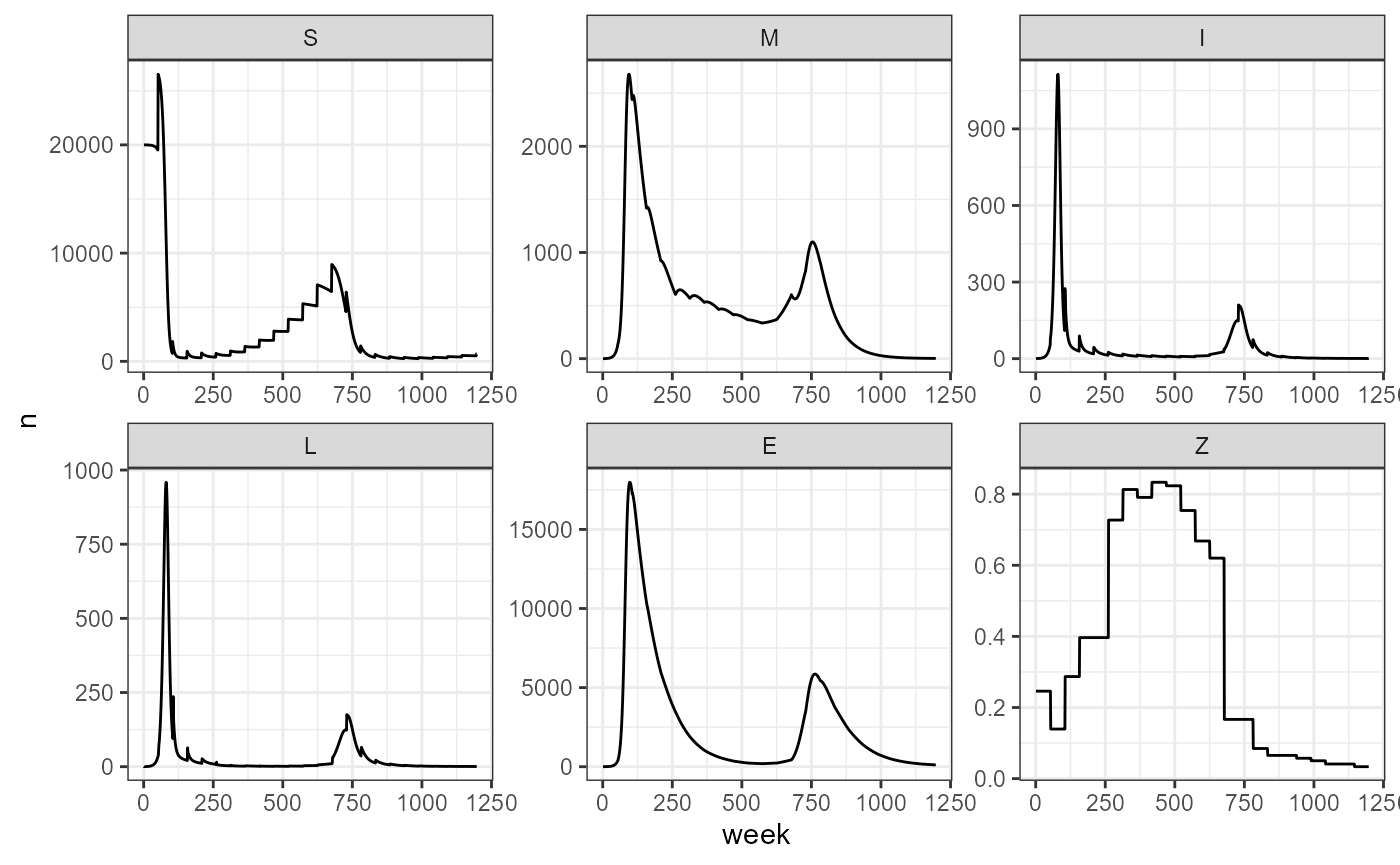
Using those parameters, this is what the underlying processes look like:
infection_probability <- lambda_t(theta=theta, tau=tau, b=b, E = vax_smile6$E[-1])
nweeks <- 1:(n_years*52)

data.frame(week = nweeks, infection_probability = infection_probability) %>%
  ggplot(aes(x = week, y = infection_probability)) +
  geom_line() +
  theme_bw() +
  labs(title = "Infection Probability", y = "lambda(t)") -> inf_prob_plot


data.frame(year = 1:n_years, vacc.pcts) %>%
  ggplot(aes(x = year, y = vacc.pcts)) +
  geom_point() +
  geom_line() +
  theme_bw() +
  labs(title = "Vaccination Rate Data", x = "Year", y = "Vax rate") +
  scale_y_continuous(labels = scales::label_percent(), limits = c(0,1)) -> vax_rates_plot

survival_prob <- 1 / (1 + exp(-(beta_0 + beta_1 * vacc.pcts)))

vax_prcnt <- seq(0, 1, 0.001)
surv_prob <- (1 / (1 + exp(-(beta_0 + beta_1 * vax_prcnt))))


data.frame(vax_prcnt, surv_prob) %>%
  ggplot(aes(x = vax_prcnt, y = surv_prob)) +
  geom_line() +
  theme_bw() +
  scale_x_continuous(labels = scales::label_percent(), breaks = seq(0, 1, 0.1)) +
  labs(x = "Vaccination rate", y = "Survival Probability") -> survival_curve_plot

# To visualize the dispersion effort, which follows a gamma distribution
# ggplot() +
#   stat_function(fun = dgamma, args = list(rate = theta, shape = tau)) +
#   lims(x = c(0, 1))

plot_grid(plot_grid(inf_prob_plot, vax_rates_plot, ncol = 2), survival_curve_plot, nrow = 2)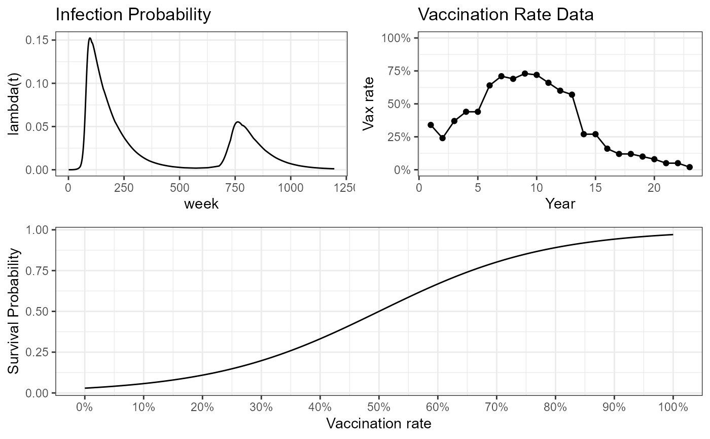
We are trying to see how our model can help us understand disease dynamics in this northern province of Vietnam. The context for these simulations then is based on the Vietnam case.
POSTER FIGURES
Vaccination
This is the survival probability curve we are assuming when incorporating vaccines. The red line shows the static 88% survival rate used in the original paper (probability of bison surviving spore exposure and developing immunity \(\zeta\)). The survival probability function used is
\[ \zeta(vax) = \frac{1}{1 + \exp^{-(\beta_0 + \beta_1 \cdot vax)}} \] We expect that every species will have a different survival probability curve, which can be adjusted through the parameters of \(\beta_0\) and \(\beta_1\). But also, different vaccine types or even different pathogen strains may have a role in this survival curve, thus parameters can be adjusted accordingly.
Survival curves
# Palette for the three scenarios
surv_palette <- viridisLite::viridis(12, option = "A")
surv_3_cols <- surv_palette[c(2,6,9)]
# scales::show_col(surv_3_cols)
my_beta_1 = 10
my_betas_0 = seq(-11, 5, length.out = 20)
sim_betas_0 <- c(-10, -3, 1.5)

vax_prcnt <- seq(0, 1, 0.001)

data.frame(vax_prcnt, betas_0 = rep(sim_betas_0, each = length(vax_prcnt)), betas_1 = my_beta_1) %>%
  mutate(surv_prob = (1 / (1 + exp(-(betas_0 + betas_1 * vax_prcnt))))) -> sim_survival_curves

data.frame(vax_prcnt, betas_0 = rep(my_betas_0, each = length(vax_prcnt)), betas_1 = my_beta_1)  %>%
  mutate(surv_prob = (1 / (1 + exp(-(betas_0 + betas_1 * vax_prcnt))))) %>%
  ggplot(aes(x = vax_prcnt, y = surv_prob, color = betas_0, fill = betas_0)) +
  geom_line(linewidth = 0.8) +
  geom_path(data = sim_survival_curves, aes(x = vax_prcnt, y = surv_prob, group = betas_0), color = "grey", linewidth = 1.5) +
  # geom_hline(yintercept = 0.88, color = "red", linewidth = 0.9) +
  scale_color_viridis_c(option = "A") +
  scale_fill_viridis_c(option = "A") +
  theme_bw() +
  scale_x_continuous(labels = scales::label_percent(), breaks = seq(0, 1, 0.1)) +
  labs(x = "Vaccination rate", y = "Survival Probability", color = expression(beta[0]),
       title = expression("Survival probability curves with fixed"~beta[1]~"=10"))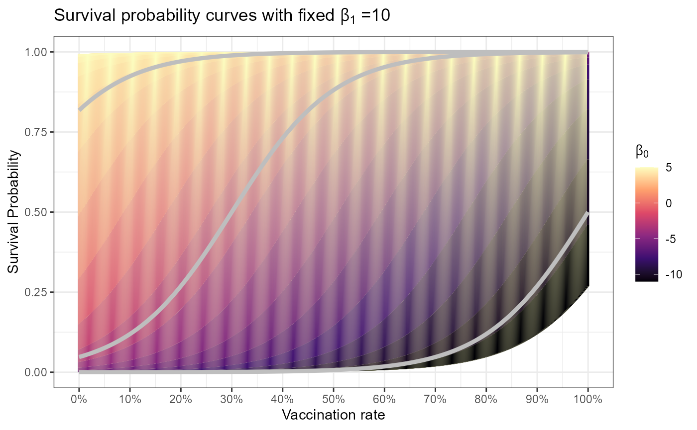
data.frame(vax_prcnt, betas_0 = rep(sim_betas_0, each = length(vax_prcnt)), betas_1 = my_beta_1) %>%
  mutate(surv_prob = (1 / (1 + exp(-(betas_0 + betas_1 * vax_prcnt))))) %>%
  mutate(betas_0 = factor(betas_0)) -> my_vax_curves

# my_vax_curves %>%
#   ggplot(aes(x = vax_prcnt, y = surv_prob, color = betas_0)) +
#   geom_line(linewidth = 1) +
#   # geom_hline(yintercept = 0.88, color = "red", linewidth = 0.9) +
#   theme_bw() +
#   scale_x_continuous(labels = scales::label_percent(), breaks = seq(0, 1, 0.1)) +
#  labs(x = "Vaccination rate", y = "Survival Probability", color = expression(beta[0]),
#        title = expression("Survival probability curves with fixed"~beta[1]~"=10")) +
#   scale_color_manual(values = surv_3_cols)
No VAX SCENARIOS
# epi poster scenario defaults
my_tau <- 1
my_theta <- 100
my_b_fixed <- 0.001

# These are the survival probabilities when there is no vaccination under those three curves.
low_surv <- my_vax_curves %>% filter(betas_0 == -10 & vax_prcnt == 0) %>%  pull(surv_prob)
med_surv <- my_vax_curves %>% filter(betas_0 == -3 & vax_prcnt == 0) %>%  pull(surv_prob)
high_surv <- my_vax_curves %>% filter(betas_0 == 1.5 & vax_prcnt == 0) %>%  pull(surv_prob)
LOW SURVIVAL
novax_noseason <- smile_main(theta = my_theta, tau = my_tau, years = 23,
                            # fixed survival probability and fixed b
                            zeta_novax = low_surv, b_fixed = my_b_fixed,
                            # parameters for host population dynamics include births and deaths
                            N1 = 20000, K = 50000, rho_pop = 0.36, sigmaa = 0.92^(1/52),
                            output_df = TRUE)

# novax_noseason %>% build_SMILE_plots()

novax_yesseason <- smile_main(theta = my_theta, tau = my_tau, years = 23,
                            # fixed survival probability
                            zeta_novax = low_surv,
                            # Parameters to induce seasonal forcing in transmission
                            b0 = -30, b1 = 0.85, period = 3*52,
                            # parameters for host population dynamics include births and deaths
                            N1 = 20000, K = 50000, rho_pop = 0.36, sigmaa = 0.92^(1/52),
                            output_df = TRUE)
# novax_yesseason %>% build_SMILE_plots()
novax_noseason %>%
  pivot_longer(-week, names_to = "compartment", values_to = "n") %>%
  mutate(compartment = factor(compartment, levels = c("S", "M", "I", "L", "E", "Z"))) %>%
  mutate(seasonality = "no") -> long_novax_noseason

novax_yesseason %>%
  pivot_longer(-week, names_to = "compartment", values_to = "n") %>%
  mutate(compartment = factor(compartment, levels = c("S", "M", "I", "L", "E", "Z"))) %>%
  mutate(seasonality = "yes") -> long_novax_yesseason

bind_rows(long_novax_noseason, long_novax_yesseason) %>%
  filter(compartment %in% c("S", "M", "L")) %>%
  mutate(cat = case_when(
    compartment == "S" ~ "S - Susceptible",
    compartment == "M" ~ "M - Immune",
    compartment == "L" ~ "L - Local Infectious Zone"
  )) %>%
  mutate(cat = factor(cat, levels = c("S - Susceptible", "M - Immune", "L - Local Infectious Zone"))) %>%
  ggplot(aes(x = week, y = n, color = seasonality)) +
  facet_wrap(~cat, scales = "free") +
  geom_line(linewidth = 0.8) +
  theme_bw() +
  scale_color_manual(values = c("#E95562FF", "#120D32FF")) +
  # scale_linetype_manual(values = c("dashed", "solid")) +
  labs(title = paste("No vaccination, low survival - zeta =", signif(low_surv, 4)),
       y = "Number of individuals")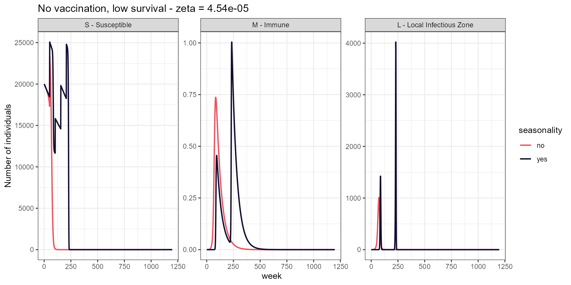
MED SURVIVAL
novax_noseason <- smile_main(theta = my_theta, tau = my_tau, years = 23,
                            # fixed survival probability and fixed b
                            zeta_novax = med_surv, b_fixed = my_b_fixed,
                            # parameters for host population dynamics include births and deaths
                            N1 = 20000, K = 50000, rho_pop = 0.36, sigmaa = 0.92^(1/52),
                            output_df = TRUE)

# novax_noseason %>% build_SMILE_plots()

novax_yesseason <- smile_main(theta = my_theta, tau = my_tau, years = 23,
                            # fixed survival probability
                            zeta_novax = med_surv,
                            # Parameters to induce seasonal forcing in transmission
                            b0 = -30, b1 = 0.85, period = 3*52,
                            # parameters for host population dynamics include births and deaths
                            N1 = 20000, K = 50000, rho_pop = 0.36, sigmaa = 0.92^(1/52),
                            output_df = TRUE)
# novax_yesseason %>% build_SMILE_plots()
novax_noseason %>%
  pivot_longer(-week, names_to = "compartment", values_to = "n") %>%
  mutate(compartment = factor(compartment, levels = c("S", "M", "I", "L", "E", "Z"))) %>%
  mutate(seasonality = "no") -> long_novax_noseason

novax_yesseason %>%
  pivot_longer(-week, names_to = "compartment", values_to = "n") %>%
  mutate(compartment = factor(compartment, levels = c("S", "M", "I", "L", "E", "Z"))) %>%
  mutate(seasonality = "yes") -> long_novax_yesseason

bind_rows(long_novax_noseason, long_novax_yesseason) %>%
  filter(compartment %in% c("S", "M", "L")) %>%
  mutate(cat = case_when(
    compartment == "S" ~ "S - Susceptible",
    compartment == "M" ~ "M - Immune",
    compartment == "L" ~ "L - Local Infectious Zone"
  )) %>%
  mutate(cat = factor(cat, levels = c("S - Susceptible", "M - Immune", "L - Local Infectious Zone"))) %>%
  ggplot(aes(x = week, y = n, color = seasonality)) +
  facet_wrap(~cat, scales = "free") +
  geom_line(linewidth = 0.8) +
  theme_bw() +
  scale_color_manual(values = c("#E95562FF", "#120D32FF")) +
  # scale_linetype_manual(values = c("dashed", "solid")) +
  labs(title = paste("No vaccination, medium survival - zeta =", signif(med_surv, 4)),
       y = "Number of individuals")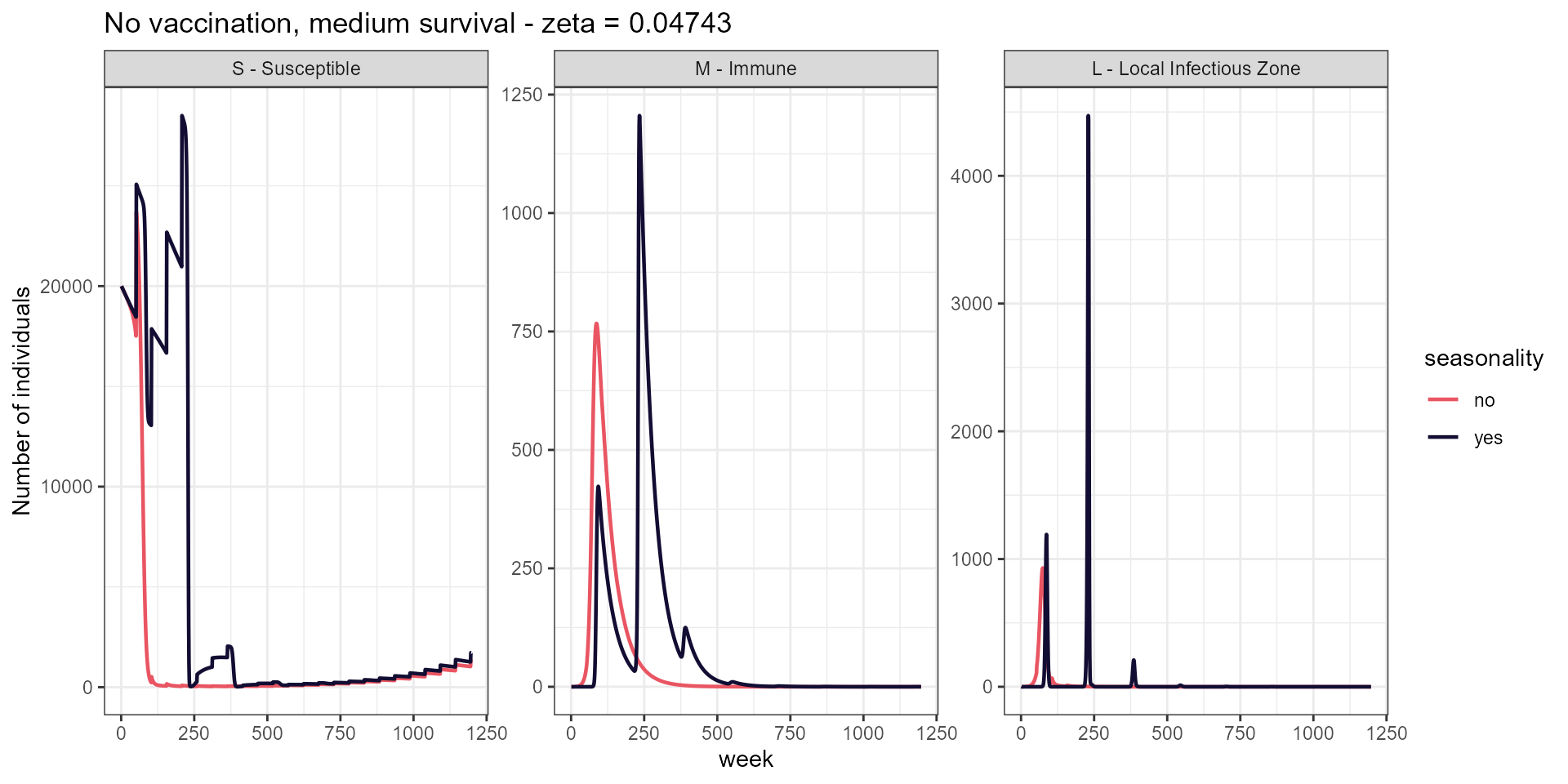
HIGH SURVIVAL
novax_noseason <- smile_main(theta = my_theta, tau = my_tau, years = 23,
                            # fixed survival probability and fixed b
                            zeta_novax = high_surv, b_fixed = my_b_fixed,
                            # parameters for host population dynamics include births and deaths
                            N1 = 20000, K = 50000, rho_pop = 0.36, sigmaa = 0.92^(1/52),
                            output_df = TRUE)

# novax_noseason %>% build_SMILE_plots()

novax_yesseason <- smile_main(theta = my_theta, tau = my_tau, years = 23,
                            # fixed survival probability
                            zeta_novax = high_surv,
                            # Parameters to induce seasonal forcing in transmission
                            b0 = -30, b1 = 0.85, period = 3*52,
                            # parameters for host population dynamics include births and deaths
                            N1 = 20000, K = 50000, rho_pop = 0.36, sigmaa = 0.92^(1/52),
                            output_df = TRUE)
# novax_yesseason %>% build_SMILE_plots()
novax_noseason %>%
  pivot_longer(-week, names_to = "compartment", values_to = "n") %>%
  mutate(compartment = factor(compartment, levels = c("S", "M", "I", "L", "E", "Z"))) %>%
  mutate(seasonality = "no") -> long_novax_noseason

novax_yesseason %>%
  pivot_longer(-week, names_to = "compartment", values_to = "n") %>%
  mutate(compartment = factor(compartment, levels = c("S", "M", "I", "L", "E", "Z"))) %>%
  mutate(seasonality = "yes") -> long_novax_yesseason

bind_rows(long_novax_noseason, long_novax_yesseason) %>%
  filter(compartment %in% c("S", "M", "L")) %>%
  mutate(cat = case_when(
    compartment == "S" ~ "S - Susceptible",
    compartment == "M" ~ "M - Immune",
    compartment == "L" ~ "L - Local Infectious Zone"
  )) %>%
  mutate(cat = factor(cat, levels = c("S - Susceptible", "M - Immune", "L - Local Infectious Zone"))) %>%
  ggplot(aes(x = week, y = n, color = seasonality)) +
  facet_wrap(~cat, scales = "free") +
  geom_line(linewidth = 0.8) +
  theme_bw() +
  scale_color_manual(values = c("#E95562FF", "#120D32FF")) +
  # scale_linetype_manual(values = c("dashed", "solid")) +
  labs(title = paste("No vaccination, high survival - zeta =", signif(high_surv, 4)),
       y = "Number of individuals")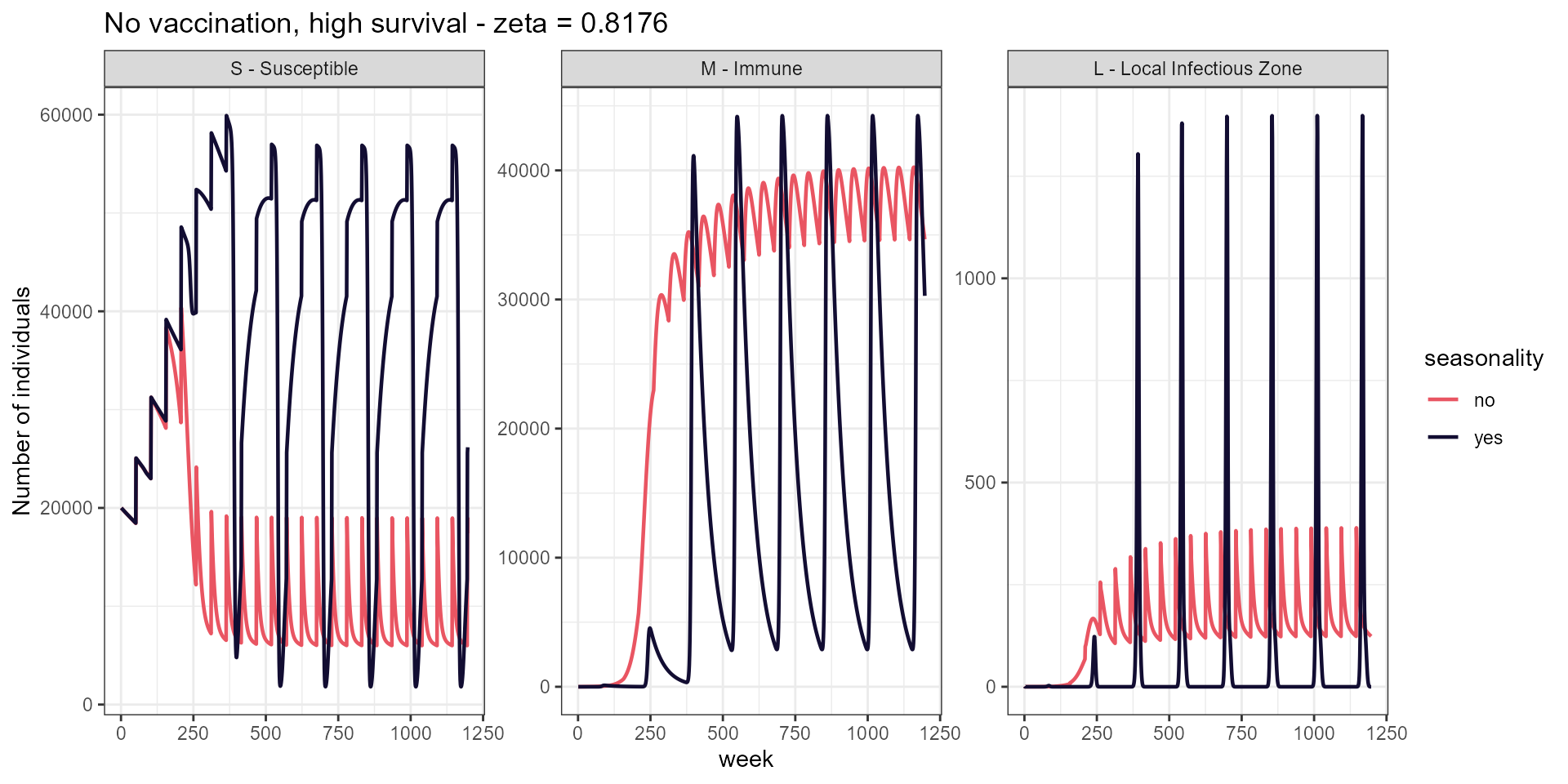
Survival probability for each year given vaccination data
vax_rates = rep(vacc.pcts, each=52)
data.frame(n_weeks = 1:(23*52), vax_rates = rep(vacc.pcts, each=52), betas_0 = rep(sim_betas_0, each = length(vax_rates)), betas_1 = my_beta_1) %>%
mutate(zeta = (1 / (1 + exp(-(betas_0 + betas_1 * vax_rates))))) %>%
mutate(betas_0 = factor(betas_0)) %>%
ggplot(aes(x = n_weeks, y = zeta, color = betas_0)) +
geom_line(linewidth = 1.2) +
# geom_hline(yintercept = 0.88, color = "red", linewidth = 0.9) +
theme_bw() +
# scale_x_continuous(labels = scales::label_percent(), breaks = seq(0, 1, 0.1)) +
labs(x = "Week", y = expression(zeta), color = expression(beta[0]),
# title = expression("Survival probability given vaccination data under three different survival curves")
) +
scale_color_manual(values = surv_3_cols)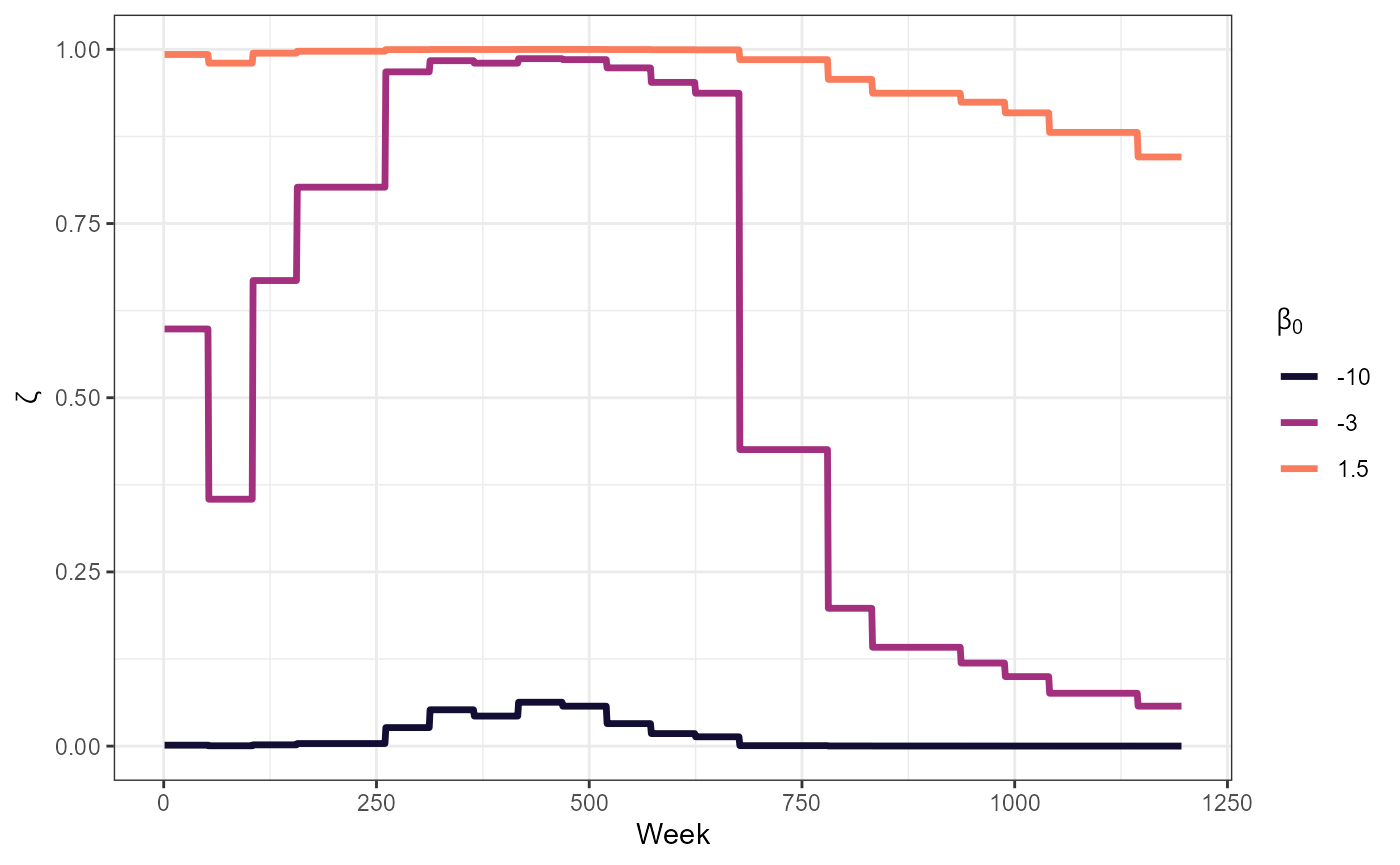 # Vietnam data
# scales::show_col(viridisLite::viridis(3, begin = 0.5, end = 0.8, option = "A"))

vietnam_data %>%
  select(year, buffalo_cases, cattle_cases, horse_cases, total_animal_cases) %>%
  mutate(year = factor(year, levels = 1991:2013)) %>%
  pivot_longer(-c(year, total_animal_cases), names_to = "species", values_to = "cases") %>%
  mutate(species = str_remove(species, "_cases")) -> case_data

vietnam_data %>%
  select(year, vaccine_coverage) %>%
  mutate(year = factor(year, levels = 1991:2013)) -> vax_data

case_data %>%
  ggplot(aes(x = year, y = cases/10)) +
  geom_col(data = vax_data, aes(x = year, y = vaccine_coverage), width = 0.5, color = "lightgrey", fill = "lightgrey") +
  geom_text(data = vax_data, aes(x = year, y = vaccine_coverage, label = paste0(round(vaccine_coverage, 2)*100, "%")), vjust = -0.5, size = 2.5) +
  geom_path(aes(color = species, group = species, linetype = species), linewidth = 1.2, alpha = 0.8) +
  theme_bw() +
  labs(y = "Vaccine coverage") +
  scale_y_continuous(label = scales::label_percent(), limits = c(0, 1), sec.axis = sec_axis(~ . * 10, name = "Number of cases", breaks = 0:10)) +
  scale_linetype_manual(values = c("solid", "longdash", "twodash")) +
  # scale_color_manual(values = c("#120D32FF", "#331068FF", "#7D2482FF")) +
  scale_color_manual(values = viridisLite::viridis(3, begin = 0.5, end = 0.8, option = "A")) +
  theme(axis.text.x = element_text(angle = 90, vjust = 0.5),
        legend.position = c(0.9, 0.85),
        legend.background = element_rect(color = "grey"),
        legend.title = element_blank())
VAX SCENARIOS
nweeks <- 23*52
my_b_season <- b_season(b0 = -30, b1 = 0.85, period = 3*52,t= 0:nweeks)
LOW SURVIVAL
vax_noseason_low_surv <- smile_main(theta = my_theta, tau = my_tau, years = 23,
                            # fixed b for no seasonality
                            b_fixed = my_b_fixed,
                            # parameters for survival curve with varying vaccination levels
                            beta_0 = -10, beta_1 = 10, vax = vacc.pcts,
                            # parameters for host population dynamics include births and deaths
                            N1 = 20000, K = 50000, rho_pop = 0.36, sigmaa = 0.92^(1/52),
                            output_df = TRUE)
plot_grid(vax_noseason_low_surv %>% build_SMILE_plots() + labs(title = "noseason-lowsurv"),
          vax_noseason_low_surv %>% build_SL_plot())
vax_season_low_surv <- smile_main(theta = my_theta, tau = my_tau, years = 23,
                            # Parameters to induce seasonal forcing in transmission
                            b0 = -30, b1 = 0.85, period = 3*52,
                            # parameters for survival curve with varying vaccination levels
                            beta_0 = -10, beta_1 = 10, vax = vacc.pcts,
                            # parameters for host population dynamics include births and deaths
                            N1 = 20000, K = 50000, rho_pop = 0.36, sigmaa = 0.92^(1/52),
                            output_df = TRUE)
plot_grid(vax_season_low_surv %>% build_SMILE_plots() + labs(title = "season-lowsurv"),
          vax_season_low_surv %>% build_SL_plot())
MED SURVIVAL
vax_noseason_med_surv <- smile_main(theta = my_theta, tau = my_tau, years = 23,
                            # fixed b for no seasonality
                            b_fixed = my_b_fixed,
                            # parameters for survival curve with varying vaccination levels
                            beta_0 = -3, beta_1 = 10, vax = vacc.pcts,
                            # parameters for host population dynamics include births and deaths
                            N1 = 20000, K = 50000, rho_pop = 0.36, sigmaa = 0.92^(1/52),
                            output_df = TRUE)
plot_grid(vax_noseason_med_surv %>% build_SMILE_plots() + labs(title = "noseason_medsurv"),
          vax_noseason_med_surv %>% build_SL_plot())
vax_season_med_surv <- smile_main(theta = my_theta, tau = my_tau, years = 23,
                            # Parameters to induce seasonal forcing in transmission
                            b0 = -30, b1 = 0.85, period = 3*52,
                            # parameters for survival curve with varying vaccination levels
                            beta_0 = -3, beta_1 = 10, vax = vacc.pcts,
                            # parameters for host population dynamics include births and deaths
                            N1 = 20000, K = 50000, rho_pop = 0.36, sigmaa = 0.92^(1/52),
                            output_df = TRUE)
plot_grid(vax_season_med_surv %>% build_SMILE_plots() + labs(title = "season_medsurv"),
          vax_season_med_surv %>% build_SL_plot())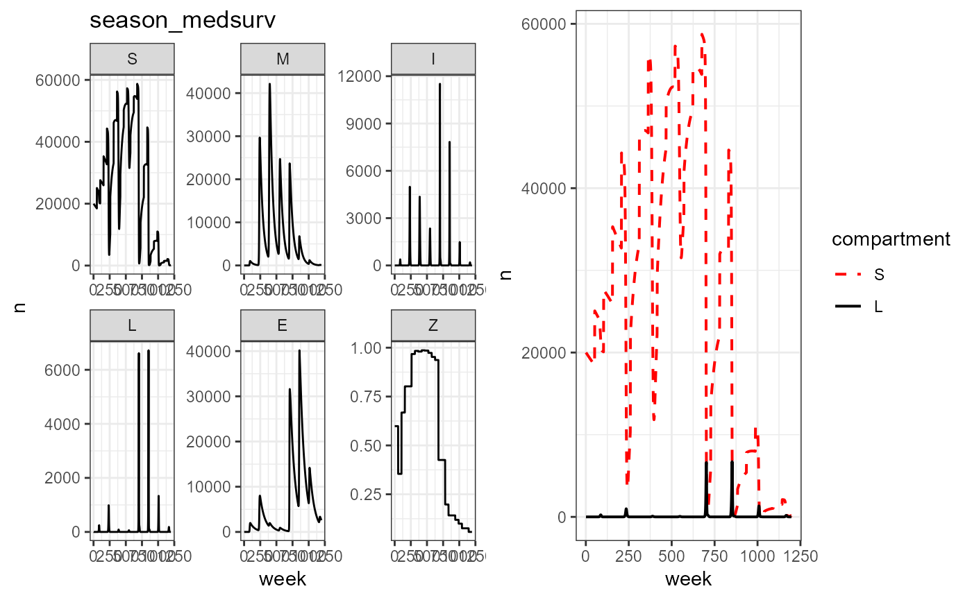
HIGH SURVIVAL
vax_noseason_high_surv <- smile_main(theta = my_theta, tau = my_tau, years = 23,
                            # fixed b for no seasonality
                            b_fixed = my_b_fixed,
                            # parameters for survival curve with varying vaccination levels
                            beta_0 = 1.5, beta_1 = 10, vax = vacc.pcts,
                            # parameters for host population dynamics include births and deaths
                            N1 = 20000, K = 50000, rho_pop = 0.36, sigmaa = 0.92^(1/52),
                            output_df = TRUE)
plot_grid(vax_noseason_high_surv %>% build_SMILE_plots() + labs(title = "noseason_highsurv"),
          vax_noseason_high_surv %>% build_SL_plot())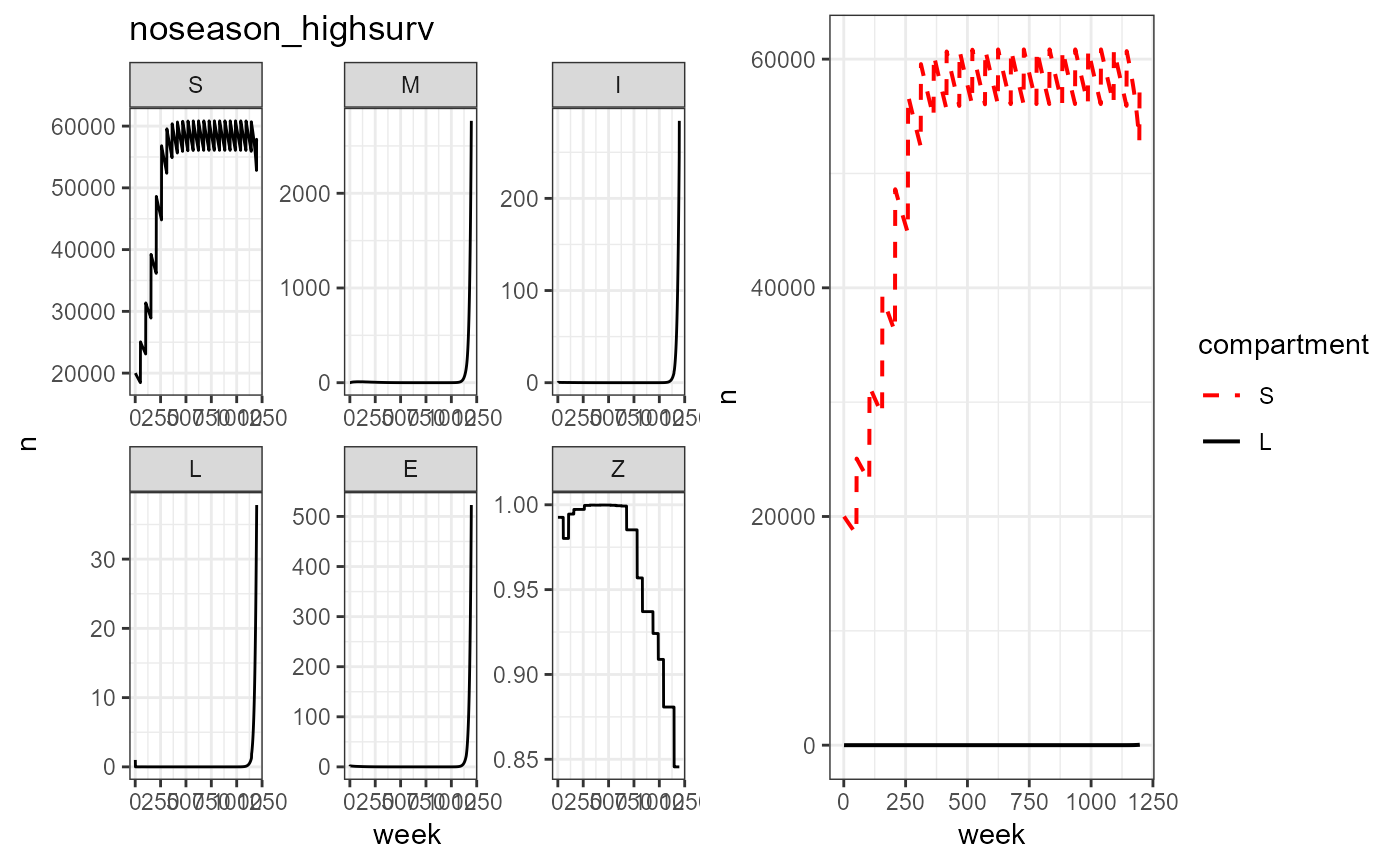
vax_season_high_surv <- smile_main(theta = my_theta, tau = my_tau, years = 23,
                            # Parameters to induce seasonal forcing in transmission
                            b0 = -30, b1 = 0.85, period = 3*52,
                            # parameters for survival curve with varying vaccination levels
                            beta_0 = 1.5, beta_1 = 10, vax = vacc.pcts,
                            # parameters for host population dynamics include births and deaths
                            N1 = 20000, K = 50000, rho_pop = 0.36, sigmaa = 0.92^(1/52),
                            output_df = TRUE)
plot_grid(vax_season_high_surv%>% build_SMILE_plots() + labs(title = "season_highsurv"),
          vax_season_high_surv%>% build_SL_plot())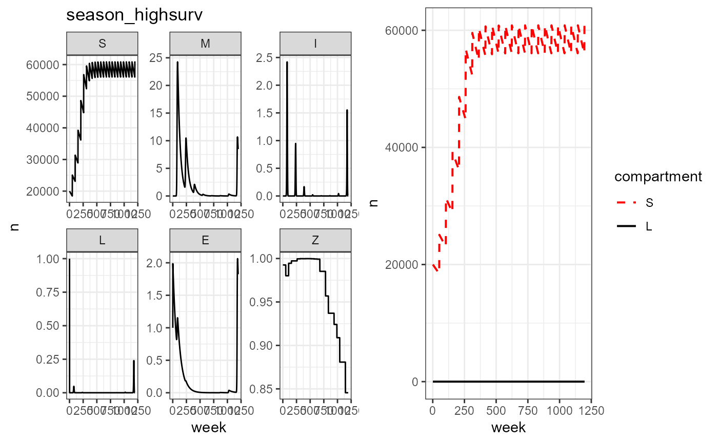
FIGS for VAX
# LOW SURV
big_df %>%
  filter(survival == "low") %>%
  filter(compartment %in% c("S", "M", "L")) %>%
  mutate(cat = case_when(
    compartment == "S" ~ "S - Susceptible",
    compartment == "M" ~ "M - Immune",
    compartment == "L" ~ "L - Local Infectious Zone"
  )) %>%
  mutate(cat = factor(cat, levels = c("S - Susceptible", "M - Immune", "L - Local Infectious Zone"))) %>%
  ggplot(aes(x = week, y = n, color = seasonality)) +
  facet_wrap(~cat, scales = "free") +
  geom_line(linewidth = 0.8) +
  theme_bw() +
  scale_color_manual(values = c("#E95562FF", "#120D32FF")) +
  # scale_linetype_manual(values = c("dashed", "solid")) +
  labs(title = "Vaccination, low survival",
       y = "Number of individuals")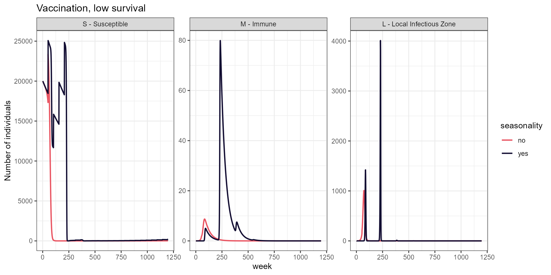
# MED SURV
big_df %>%
  filter(survival == "med") %>%
  filter(compartment %in% c("S", "M", "L")) %>%
  mutate(cat = case_when(
    compartment == "S" ~ "S - Susceptible",
    compartment == "M" ~ "M - Immune",
    compartment == "L" ~ "L - Local Infectious Zone"
  )) %>%
  mutate(cat = factor(cat, levels = c("S - Susceptible", "M - Immune", "L - Local Infectious Zone"))) %>%
  ggplot(aes(x = week, y = n, color = seasonality)) +
  facet_wrap(~cat, scales = "free") +
  geom_line(linewidth = 0.8) +
  theme_bw() +
  scale_color_manual(values = c("#E95562FF", "#120D32FF")) +
  # scale_linetype_manual(values = c("dashed", "solid")) +
  labs(title = "Vaccination, med survival",
       y = "Number of individuals")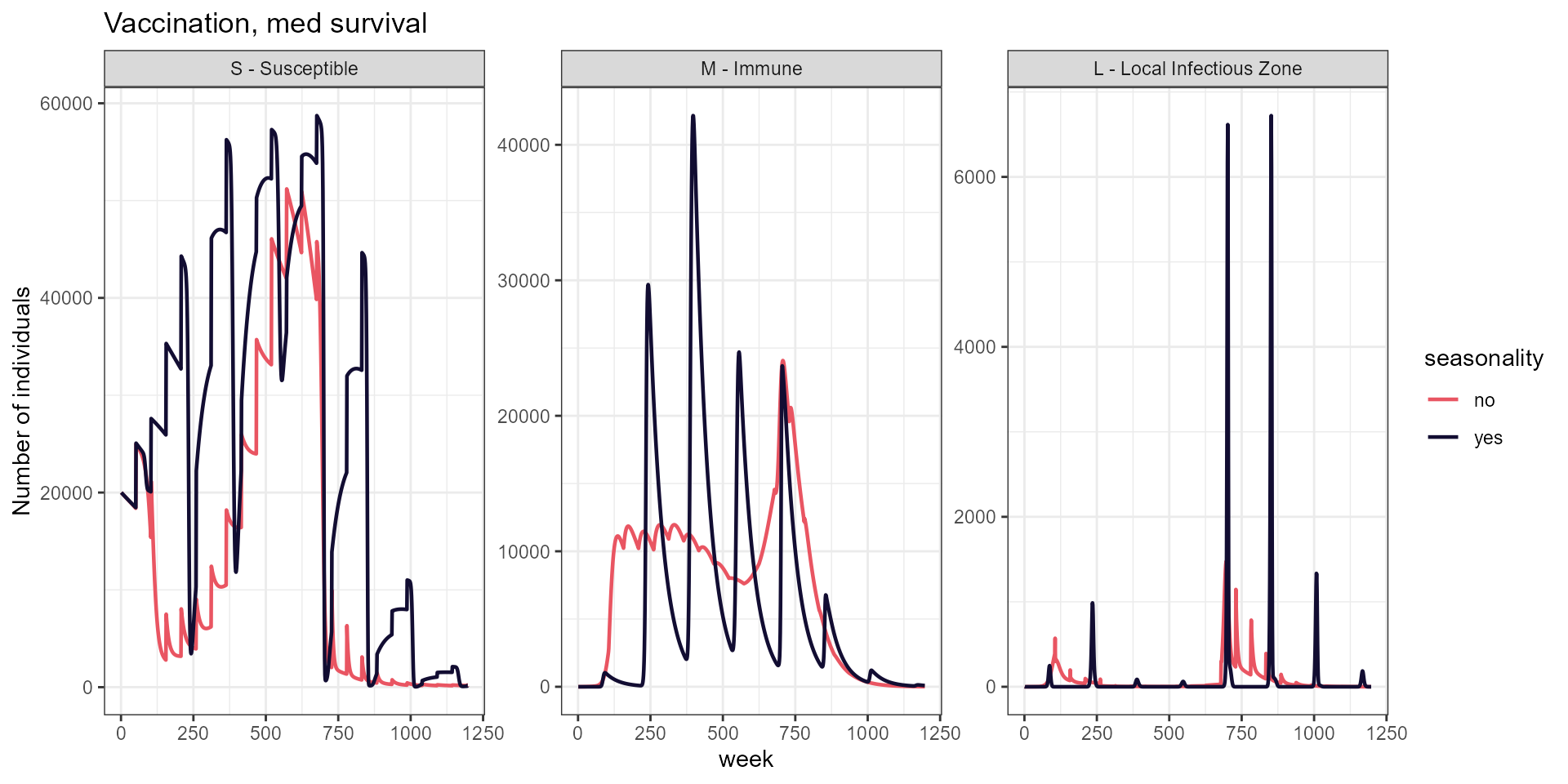
# HIGH SURV
big_df %>%
  filter(survival == "high") %>%
  filter(compartment %in% c("S", "M", "L")) %>%
  mutate(cat = case_when(
    compartment == "S" ~ "S - Susceptible",
    compartment == "M" ~ "M - Immune",
    compartment == "L" ~ "L - Local Infectious Zone"
  )) %>%
  mutate(cat = factor(cat, levels = c("S - Susceptible", "M - Immune", "L - Local Infectious Zone"))) %>%
  ggplot(aes(x = week, y = n, color = seasonality)) +
  facet_wrap(~cat, scales = "free") +
  geom_line(linewidth = 0.8) +
  theme_bw() +
  scale_color_manual(values = c("#E95562FF", "#120D32FF")) +
  # scale_linetype_manual(values = c("dashed", "solid")) +
  labs(title = "Vaccination, high survival",
       y = "Number of individuals")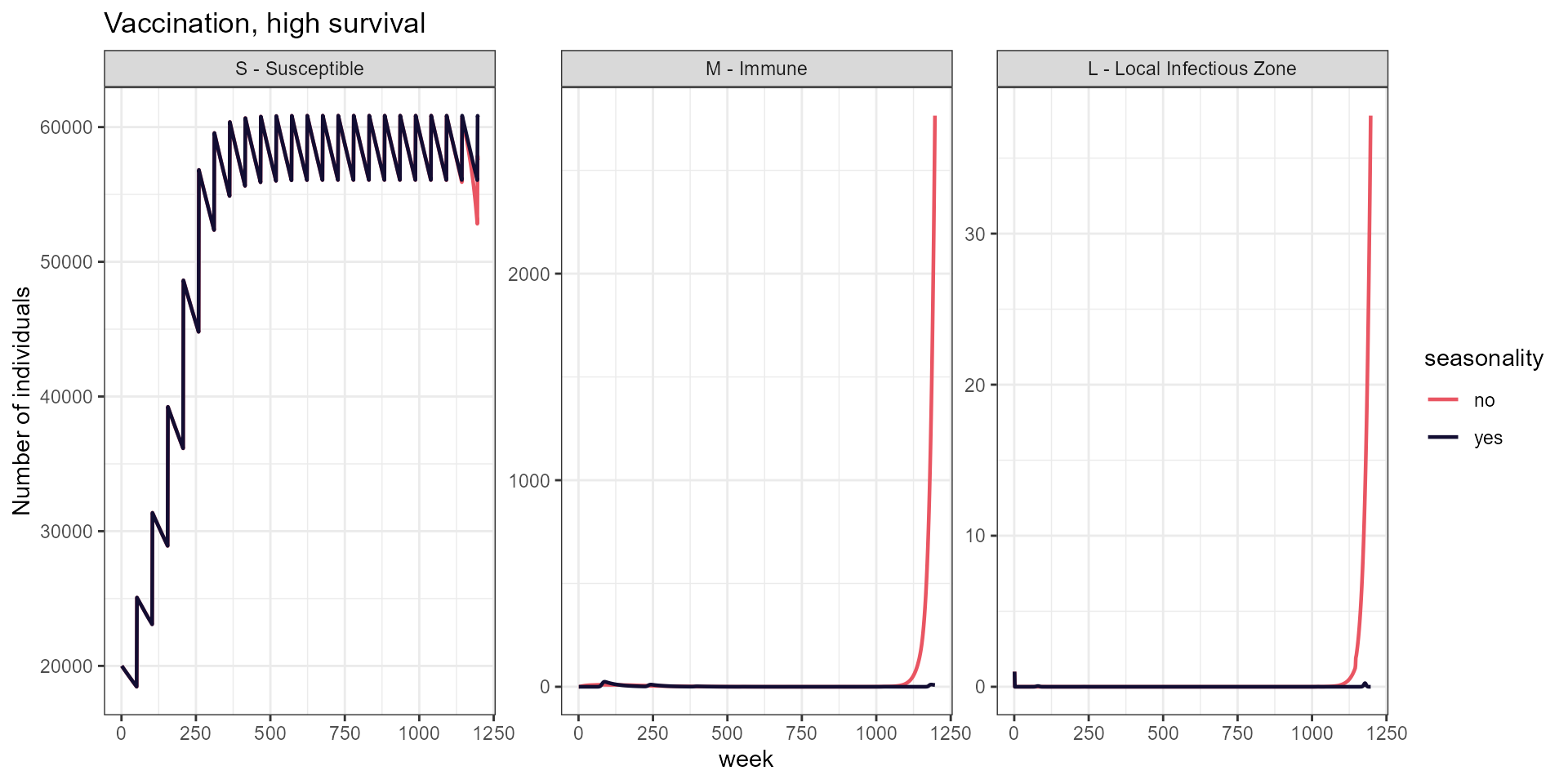
big_df %>%
  mutate(survival = factor(survival, levels = c("low", "med", "high"))) %>%
  filter(compartment %in% c("S", "M", "L")) %>%
  filter(seasonality == "no") %>%
    mutate(cat = case_when(
    compartment == "S" ~ "S - Susceptible",
    compartment == "M" ~ "M - Immune",
    compartment == "L" ~ "L - Local Infectious Zone"
  )) %>%
  mutate(cat = factor(cat, levels = c("S - Susceptible", "M - Immune", "L - Local Infectious Zone"))) %>%
  ggplot(aes(x = week, y = n, color = survival)) +
  facet_wrap(~cat, scales = "free") +
  geom_line(linewidth = 0.8, alpha = 0.8) +
  theme_bw() +
  # scale_color_manual(values = c("#E95562FF", "#120D32FF")) +
  # scale_linetype_manual(values = c("dashed", "solid")) +
  labs(y = "Number of individuals", title = "No seasonal forcing") +
  scale_color_manual(values = surv_3_cols)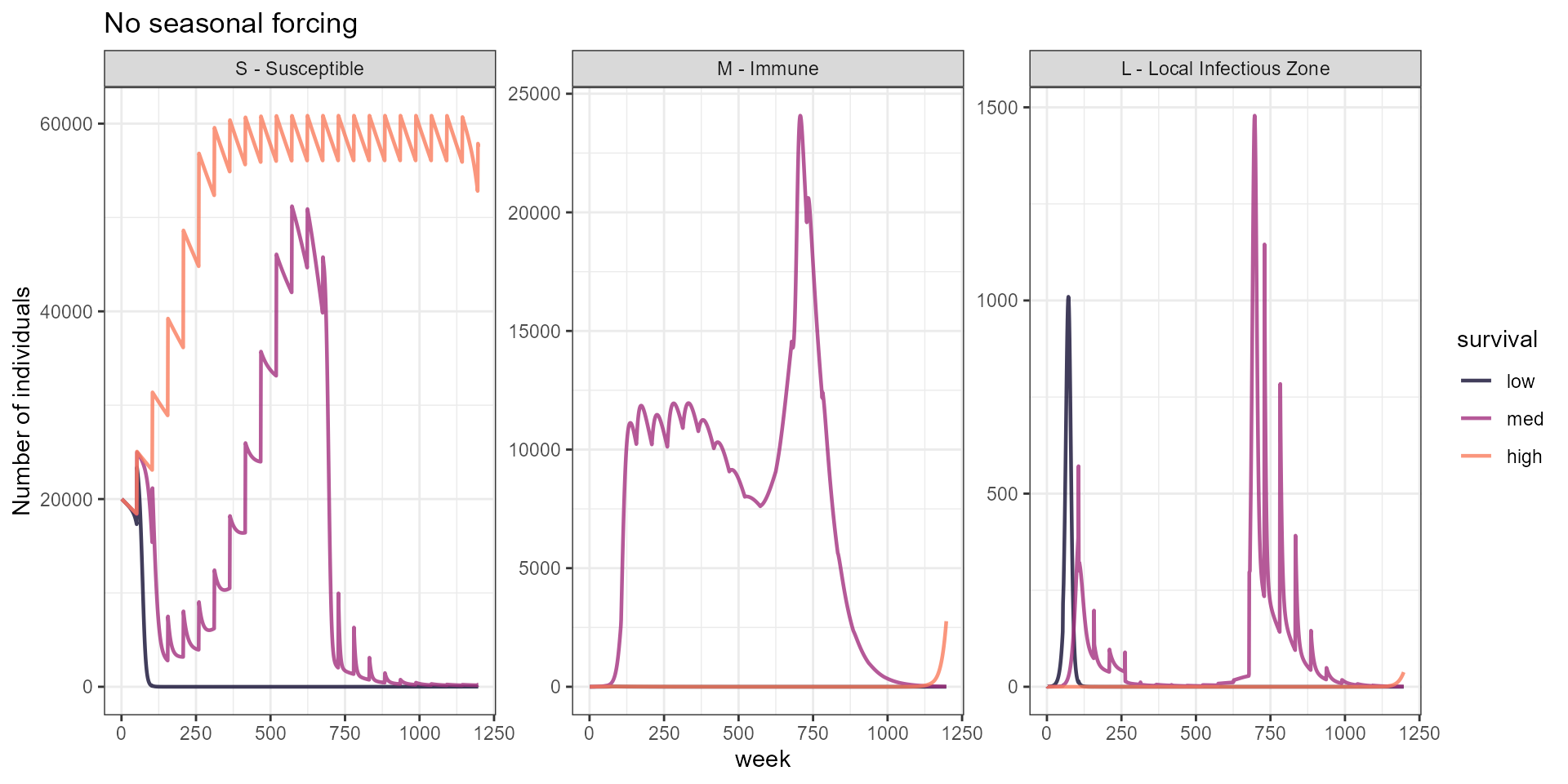
big_df %>%
  mutate(survival = factor(survival, levels = c("low", "med", "high"))) %>%
  filter(compartment %in% c("S", "M", "L")) %>%
  filter(seasonality == "yes") %>%
    mutate(cat = case_when(
    compartment == "S" ~ "S - Susceptible",
    compartment == "M" ~ "M - Immune",
    compartment == "L" ~ "L - Local Infectious Zone"
  )) %>%
  mutate(cat = factor(cat, levels = c("S - Susceptible", "M - Immune", "L - Local Infectious Zone"))) %>%
  ggplot(aes(x = week, y = n, color = survival)) +
  facet_wrap(~cat, scales = "free") +
  geom_line(linewidth = 0.8, alpha = 0.8) +
  theme_bw() +
  # scale_color_manual(values = c("#E95562FF", "#120D32FF")) +
  # scale_linetype_manual(values = c("dashed", "solid")) +
  labs(y = "Number of individuals", title = "With seasonal forcing") +
  scale_color_manual(values = surv_3_cols)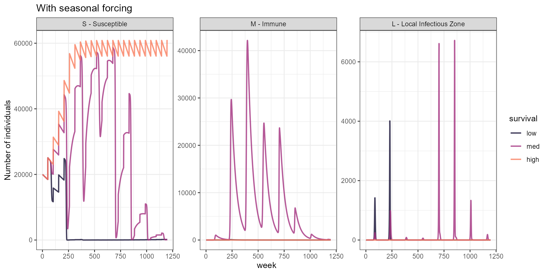
big_df_R0 %>%
  filter(seasonality == "no") %>%
  # pivot_wider(names_from = compartment, values_from = n) %>%
  # mutate(survival = factor(survival, levels = c("low", "med", "high"))) %>%
  # select(week, seasonality, survival, E) %>%
  # mutate(R0 = calc_local_R0(tau = my_tau, theta = my_theta, b = my_b_fixed, E = E)) %>%
  ggplot(aes(x = week, y = R0, color = survival)) +
  # geom_point() +
  geom_line(linewidth = 1) +
  theme_bw() +
  labs(title = "Local R0 - no seasonality") +
  scale_color_manual(values = surv_3_cols)


big_df_R0 %>%
  filter(seasonality == "yes") %>%
  # pivot_wider(names_from = compartment, values_from = n) %>%
  # mutate(survival = factor(survival, levels = c("low", "med", "high"))) %>%
  # select(week, seasonality, survival, E) %>%
  # mutate(R0 = calc_local_R0(tau = my_tau, theta = my_theta, b = my_b_fixed, E = E)) %>%
  ggplot(aes(x = week, y = R0, color = survival)) +
  # geom_point() +
  geom_line(linewidth = 1) +
  theme_bw() +
  labs(title = "Local R0 - seasonal forcing") +
  scale_color_manual(values = surv_3_cols)
big_df_R0 %>%
  mutate(season = case_when(
    seasonality == "no" ~ "No seasonal transmission",
    seasonality == "yes"~ "Seasonal forcing"
  )) %>%
  mutate(survival = factor(survival, levels = c("low", "med", "high"))) %>%
  ggplot(aes(x = week, y = R0, color = survival)) +
  facet_wrap(~season, ncol = 1, scales = "free") +
  geom_line(linewidth = 1) +
  theme_bw() +
  scale_color_manual(values = surv_3_cols) +
  theme(legend.position = "bottom")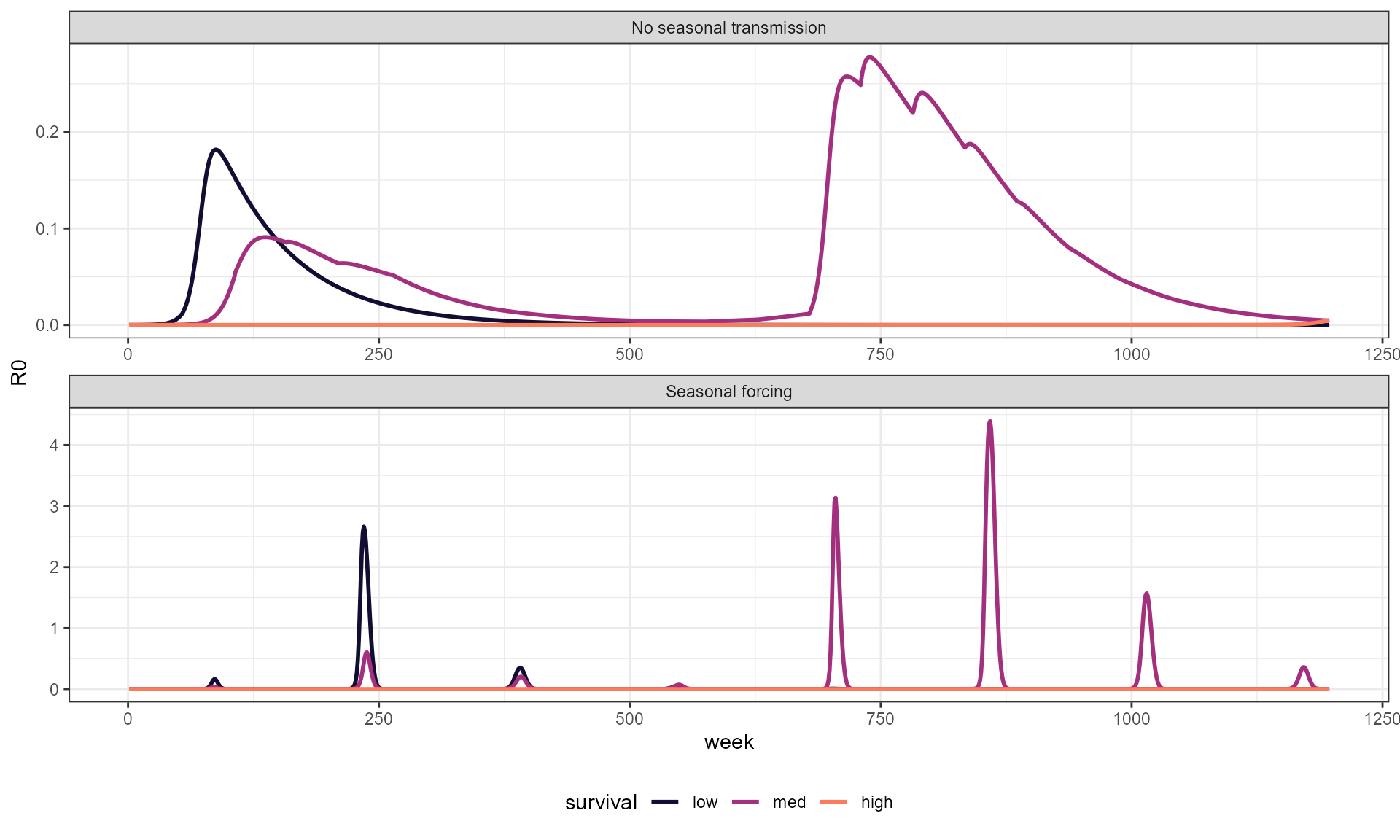
big_df %>%
  mutate(survival = factor(survival, levels = c("low", "med", "high"))) %>%
  filter(compartment %in% c("S", "L")) %>%
  ggplot(aes(x = week, y = n, color = compartment, linetype = compartment)) +
  facet_wrap(seasonality~survival, scales = "free") +
  geom_path(linewidth = 0.7) +
  theme_bw() +
  scale_color_manual(values = c("red", "black")) +
  scale_linetype_manual(values = c("dashed", "solid"))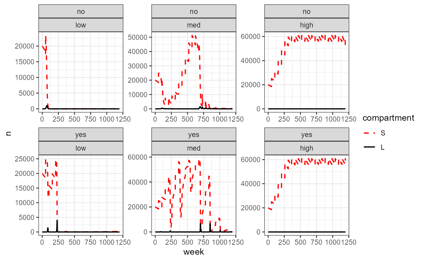
Tests —————————-
We start with a 20,000 susceptible population, but since there are no host dynamics, no reproduction, then the population just continues to decrease as a result of the outbreak. In this case, we have incorporated a high survival probability, exploring the range from 0.85 to 1, the lower the survival probability, the faster this decline in population size.
surv_prob_seq <- seq(0.85, 0.98, by = 0.01)

my_smile_df <- NULL
for(i in 1:length(surv_prob_seq)) {

  i_survival <- surv_prob_seq[i]
  sim <- smile_main(tau = 10, theta = 100, b_fixed = 0.001, years = 20, age_struc = FALSE, N1 = 20000, zeta_novax = i_survival, output_df = TRUE) %>%
    mutate(survival = i_survival)

  my_smile_df <- bind_rows(my_smile_df, sim)
}


 my_smile_df %>%
    pivot_longer(-c(week, survival), names_to = "compartment", values_to = "n") %>%
    mutate(compartment = factor(compartment, levels = c("S", "M", "I", "L", "E", "Z"))) %>%
    ggplot(aes(x = week, y = n, color = survival, group = survival)) +
    facet_wrap(~compartment, scales = "free", nrow = 1) +
    geom_line(linewidth = 1, alpha = 0.5) +
    theme_bw() +
   scale_color_viridis_c()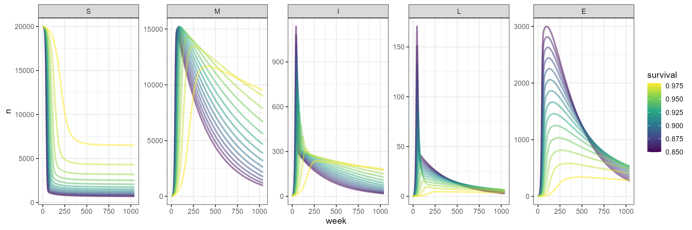
Now we consider with population dynamics, where there is a yearly birth pulse, and we have death by other causes aside from just disease. Since we still have a relatively high survival probability, you will see that outbreaks occur yearly, following the birth pulses. Over time, the population tries to settle close to carrying capacity with yearly outbreaks.
surv_prob_seq <- seq(0.85, 0.98, by = 0.01)

my_smile_df <- NULL
for(i in 1:length(surv_prob_seq)) {

  i_survival <- surv_prob_seq[i]
  sim <- smile_main(tau = 10, theta = 100, b_fixed = 0.001, years = 20, age_struc = TRUE, N1 = 20000, K =10000, rho_pop = 0.36, sigmaa = 0.92^(1/52),
                  zeta_novax = i_survival, output_df = TRUE) %>%
    mutate(survival = i_survival)

  my_smile_df <- bind_rows(my_smile_df, sim)
}


 my_smile_df %>%
   mutate(N = S + M) %>%
    pivot_longer(-c(week, survival), names_to = "compartment", values_to = "n") %>%
    mutate(compartment = factor(compartment, levels = c("S", "M", "I", "L", "E", "N"))) %>%
    ggplot(aes(x = week, y = n, color = survival, group = survival)) +
    facet_wrap(~compartment, scales = "free", nrow = 1) +
    geom_line(linewidth = 1, alpha = 0.5) +
    theme_bw() +
   scale_color_viridis_c() +
   labs(title = "K =10,000")
surv_prob_seq <- seq(0.85, 0.98, by = 0.01)

my_smile_df <- NULL
for(i in 1:length(surv_prob_seq)) {

  i_survival <- surv_prob_seq[i]
  sim <- smile_main(tau = 10, theta = 100, b_fixed = 0.001, years = 20, age_struc = TRUE, N1 = 20000, K =20000, rho_pop = 0.36, sigmaa = 0.92^(1/52),
                  zeta_novax = i_survival, output_df = TRUE) %>%
    mutate(survival = i_survival)

  my_smile_df <- bind_rows(my_smile_df, sim)
}


 my_smile_df %>%
   mutate(N = S + M) %>%
    pivot_longer(-c(week, survival), names_to = "compartment", values_to = "n") %>%
    mutate(compartment = factor(compartment, levels = c("S", "M", "I", "L", "E", "N"))) %>%
    ggplot(aes(x = week, y = n, color = survival, group = survival)) +
    facet_wrap(~compartment, scales = "free", nrow = 1) +
    geom_line(linewidth = 1, alpha = 0.5) +
    theme_bw() +
   scale_color_viridis_c() +
   labs(title = "K =20,000")
surv_prob_seq <- seq(0.85, 0.98, by = 0.01)

my_smile_df <- NULL
for(i in 1:length(surv_prob_seq)) {

  i_survival <- surv_prob_seq[i]
  sim <- smile_main(tau = 10, theta = 100, b_fixed = 0.001, years = 20, age_struc = TRUE, N1 = 20000, K =50000, rho_pop = 0.36, sigmaa = 0.92^(1/52),
                  zeta_novax = i_survival, output_df = TRUE) %>%
    mutate(survival = i_survival)

  my_smile_df <- bind_rows(my_smile_df, sim)
}


 my_smile_df %>%
   mutate(N = S + M) %>%
    pivot_longer(-c(week, survival), names_to = "compartment", values_to = "n") %>%
    mutate(compartment = factor(compartment, levels = c("S", "M", "I", "L", "E", "N"))) %>%
    ggplot(aes(x = week, y = n, color = survival, group = survival)) +
    facet_wrap(~compartment, scales = "free", nrow = 1) +
    geom_line(linewidth = 1, alpha = 0.5) +
    theme_bw() +
   scale_color_viridis_c() +
   labs(title = "K =50,000")
Now we incorporate seasonal transmission to the population. Given the 20 year time frame, we see that a K-=50,000 the population hasn’t reached it’s equilibrium yet, so we will stick to a K=20,000 to test the seasonal transmission. In this case, population dynamics and survival don’t play such a big role in outbreak timing, and we see that outbreaks are mainly dominated by the period in the seasonal transmission equation. Outbreaks are also larger, with the number of infecteds and deaths almost double what we saw in the scenarios with host dynamics and no seasonal forcing. The number of deaths is variable and changes according to the survival probability.
surv_prob_seq <- seq(0.85, 0.98, by = 0.01)

my_smile_df <- NULL
for(i in 1:length(surv_prob_seq)) {

  i_survival <- surv_prob_seq[i]
  sim <- smile_main(tau = 10, theta = 100, years = 20, age_struc = TRUE, N1 = 20000, K =20000, rho_pop = 0.36, sigmaa = 0.92^(1/52),
                  b0 = -30, b1 = 0.85, period = 3*52,
                  zeta_novax = i_survival, output_df = TRUE) %>%
    mutate(survival = i_survival)

  my_smile_df <- bind_rows(my_smile_df, sim)
}


 my_smile_df %>%
   mutate(N = S + M) %>%
    pivot_longer(-c(week, survival), names_to = "compartment", values_to = "n") %>%
    mutate(compartment = factor(compartment, levels = c("S", "M", "I", "L", "E", "N"))) %>%
    ggplot(aes(x = week, y = n, color = survival, group = survival)) +
    facet_wrap(~compartment, scales = "free", nrow = 1) +
    geom_line(linewidth = 1, alpha = 0.5) +
    theme_bw() +
   scale_color_viridis_c() +
   labs(title = "b0 = -30, b1 = 0.85, period = 3*52")
We observe with this example how the period for seasonal transmission determines the outbreaks. It would be interesting to consider different types of outbreaks, perhaps thinking about dormant spores causing outbreaks 5+ years after the animal dies.
surv_prob_seq <- seq(0.85, 0.98, by = 0.01)

my_smile_df <- NULL
for(i in 1:length(surv_prob_seq)) {

  i_survival <- surv_prob_seq[i]
  sim <- smile_main(tau = 10, theta = 100, years = 20, age_struc = TRUE, N1 = 20000, K =20000, rho_pop = 0.36, sigmaa = 0.92^(1/52),
                  b0 = -30, b1 = 0.85, period = 7*52,
                  zeta_novax = i_survival, output_df = TRUE) %>%
    mutate(survival = i_survival)

  my_smile_df <- bind_rows(my_smile_df, sim)
}


 my_smile_df %>%
   mutate(N = S + M) %>%
    pivot_longer(-c(week, survival), names_to = "compartment", values_to = "n") %>%
    mutate(compartment = factor(compartment, levels = c("S", "M", "I", "L", "E", "N"))) %>%
    ggplot(aes(x = week, y = n, color = survival, group = survival)) +
    facet_wrap(~compartment, scales = "free", nrow = 1) +
    geom_line(linewidth = 1, alpha = 0.5) +
    theme_bw() +
   scale_color_viridis_c() +
   labs(title = "b0 = -30, b1 = 0.85, period = 7*52")
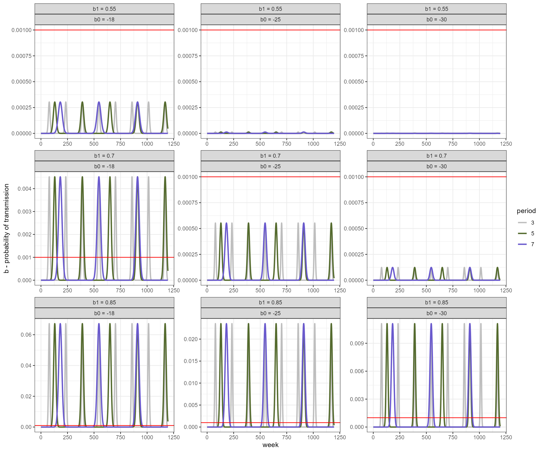
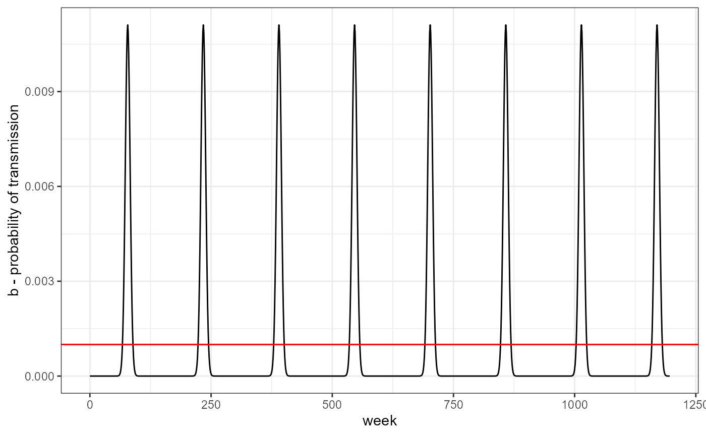
changing the parameters of the seasonal transmission function results in changes to the amplitude of the oscillations. The red line is the value used for no seasonality.
my_b_season <- b_season(b0 = -16, b1 = 0.6, period = 3*52,t= 0:nweeks)

data.frame(week = 0:nweeks, b = my_b_season) %>%
  ggplot(aes(x = week, y = b)) +
  geom_path() +
  geom_hline(yintercept = my_b_fixed, color = "red") +
  theme_bw() +
  labs(y = "b - probability of transmission")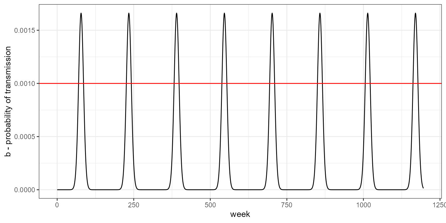
my_b0s <- c(-30, -25, -18)
my_b1s <- c(0.85, 0.7, 0.55)
period <- c(3,5, 7)

# we have 18 parameter combinations

expand.grid(my_b0s, my_b1s, period) %>%
  set_names(., c("b0", "b1", "period")) %>%
  mutate(b = pmap(list(b0, b1, period), function(x,y,z) b_season(x,y,z*52, 0:nweeks))) %>%
  unnest(cols = c(b)) %>%
  mutate(params = paste0("b0=", b0, ",b1=", b1, ",period=", period)) %>%
  mutate(week = rep(0:nweeks, 27),
         period = factor(period, levels = c(3,5, 7))) -> b_season_df

b_season_df %>%
  # filter(b1 == 0.6) %>%
  mutate(b0 = paste("b0 =", b0),
         b1 = paste("b1 =", b1)) %>%
  ggplot(aes(x = week, y = b, group = params, color = period)) +
  facet_wrap(vars(b1, b0), ncol = 3, scales = "free") +
  geom_line(linewidth = 1) +
  geom_hline(yintercept = my_b_fixed, color = "red") +
  theme_bw() +
  labs(y = "b - probability of transmission") +
  scale_color_manual(values = c("grey", "darkolivegreen", "slateblue"))