main_function
main_function.RmdIntro
Start by loading our package. In this article we want to show how the
updated function works to recreate the same simulation scenarios tested
in the first iteration of this code. Previously, multiple functions were
needed to incorporate population dynamics or seasonality, or both. In
this example, we will show you how to set the parameters to the
package’s main function SMILE::smile_main() and generate
the same scenarios as before.
The following packages are only needed for visualization and data wrangling purposes:
The original code is found in the first commit for this repository with the defined functions to evaluate the model under different assumptions of population dynamics or seasonal forcing. This is code show in also shown before each of the scenarios.
# OG functions

# Author: Juan Pablo Gomez
# Version 1.1.
# Last revised: March 7 2018.

#################################
# Infection probability based on Ponciano and Capistran 2011.
lambda.t    <-  function(theta,tau,b,E){

    1-(theta/(theta+b*E))^tau

}

# Introducing seasonality in the infection probability through b.

b.season    <-  function(b0,b1,period,t){

    exp(b0*(1+b1*cos((2*pi*t)/period)))

}

# Density dependent reproduction

rho.n   <-  function(N){

    0.41/(1+(N/5000)^(10))

}

# First case of R0

r0  <-  function(b,E,theta,tau){

    (b*E*tau)/theta

}

# Function to simulate climatic variable
# a = upper asymptote
# c = lower asymptote
# b = time required to reach half of the climatic maxima
# d = time at which the mid point between max and minimum climate is reached.
clim.func   <-  function(a,c,d,d2,b,b2,t,sd){

    if(missing(b2)){b2 <- b}
    if(missing(c)){c<-0}

    det.clim    <-   ((a-c)/(1+exp((d-t)/b)) - (a-c)/(1+exp((d2-t)/b2))) + c
    rand.clim   <-  rnorm(length(t),det.clim,sd=sd)
    return(rand.clim)

}

# Function used to estimate seasonality in infection probability using climatic variables
# wt.bar = mean of climatic covariable
# b0 = as in b.season
# b1 = as in b.season
# kw = scaling coefficient
# t = time
# period = as in b.season

infect2clim <-  function(wt.bar,b0,b1,kw,t,period){

    wt.bar + ((b0*b1)/kw)*cos((2*pi*t)/period)

}
smile1
No age structuring, infection probability is not seasonal
# Function of SMILE without any age structuring
# This is the most basic SMILE function in which I have assumed no population dynamics
# and no deaths other than disease related.
# Fixed parameters are:
# alpha= 1/52 Probability of an immune individual to become Suceptible
# zeta = 0.88 Probability that an Infected individual becomes immune
# gamma= 0.9868 Spore decay probability
# psi = 1 Number of spores in one LIZ

# Variable parameters
# b: Number of infections caused by one LIZ if there was no dispersion effort
# tau and theta: Shape and Rate parameters of the gamma distribution defining dispersion effort.

smile1  <-  function(b,theta,tau,years){

    # Fixed parameters
    alpha   <-  1/52
    zeta    <-  0.88
    gamma   <-  0.9868
    psi     <-  1

    n.weeks     <-  years*52 + 1
    S<- M<- I<- L<-E <-N<-lambda<- array(0,dim=c(n.weeks),dimnames=list(1:(n.weeks)))
    N[1]        <-  5000
    S[1]        <-  N[1]

    L[1]    <-  1; E[1] <-  L[1]*psi

    for(t in 2:n.weeks){

        tm1 <-  t-1
        lambda[tm1] <-  lambda.t(theta=theta,tau=tau,b=b,E=E[tm1])

        S[t]    <-  (S[tm1]*(1-lambda[tm1])) + M[tm1]*1/52
        I[t]    <-  S[tm1]*lambda[tm1]
        M[t]    <-  I[tm1]*zeta + M[tm1]*(1-(1/52))
        L[t]    <-  I[tm1]*(1-zeta)
        E[t]    <-  psi*L[tm1] + E[tm1]*gamma
        N[t]    <-  S[t]+M[t]

    }


    results     <-  list(Suceptibles=S[-1]
                        ,Immune=M[-1]
                        ,Infected=I[-1]
                        ,LIZ=L[-1]
                        ,Environment=E[-1]
                        ,lambda=lambda[-1])

    return(results)
}
tau=10
b=0.001

# Case 1.0: Low Dispersion. Mean dispersion effort is 0.1
theta=100
sim1.0  <-  smile1(b=b,tau=tau,theta=theta,years=10)
To recreate this scenario with the new function, we use the following
parameters. Note the argument age_struc is set to
FALSE.
sim1_1 <- smile_main(tau = tau, b_fixed = b, theta = theta, years = 10, age_struc = FALSE)
# sim1_1 <- smile_main(tau = 10, b_fixed = 0.001, theta = 100, years = 10, age_struc = FALSE)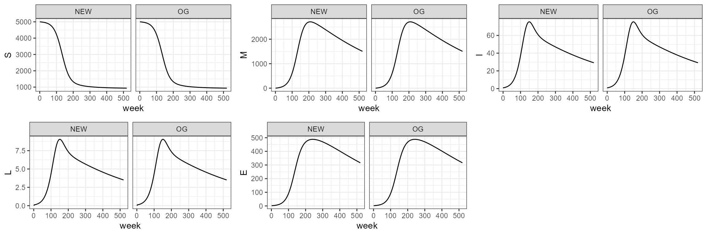
smile2
This function simulates anthrax disease dynamics without host population dynamics but infection probability has seasonal forcing.
# This function simulates anthrax disease dynamics without host population dynamics
# but infection probability has seasonal forcing.
# Fixed parameter are the same as in smile1 function.
# Variable parameters tau and theta are also the same and b0, b1 and period
# introduce seasonality to the infection probability by modifying b. In this function
# I assume that seasonality is product of an exponential cosine function where the intensity
# of the seasonality is given by b0*b1 and period gives the periodicity of the outbreak
# tau and theta: Shape and Rate parameters of the gamma distribution defining dispersion effort.
# period: is the period in weeks of the exponential sinusoid function

smile2  <-  function(b0,b1,period,theta,tau,years){

    # Fixed parameters
    alpha   <-  1/52
    zeta    <-  0.88
    gamma   <-  0.9868
    psi     <-  1

    n.weeks     <-  years*52 + 1
    S<- M<- I<- L<-E <-N<-lambda<- array(0,dim=c(n.weeks),dimnames=list(1:(n.weeks)))
    N[1]        <-  5000
    S[1]        <-  N[1]

    L[1]    <-  1; E[1] <-  L[1]*psi

    for(t in 2:n.weeks){

        tm1 <-  t-1
        b   <-  b.season(b0=b0,b1=b1,period=period,t=t)
        lambda[tm1] <-  lambda.t(theta=theta,tau=tau,b=b,E=E[tm1])

        S[t]    <-  (S[tm1]*(1-lambda[tm1])) + M[tm1]*1/52
        I[t]    <-  S[tm1]*lambda[tm1]
        M[t]    <-  I[tm1]*zeta + M[tm1]*(1-(1/52))
        L[t]    <-  I[tm1]*(1-zeta)
        E[t]    <-  psi*L[tm1] + E[tm1]*gamma
        N[t]    <-  S[t]+M[t]

    }


    results     <-  list(Suceptibles=S[-1]
                        ,Immune=M[-1]
                        ,Infected=I[-1]
                        ,LIZ=L[-1]
                        ,Environment=E[-1]
                        ,lambda=lambda[-1])

    return(results)
}
# Case 2: No age structuring, infection probability has seasonal forcing
tau=10
b0=-30
b1=0.85
period=3*52

# Case 2.0: Low dispersion
theta=100
sim2.0  <-  smile2(b0=b0,b1=b1,period=period,tau=tau,theta=theta,years=10)
sim2_1 <- smile_main(b0 = b0, b1 = b1, period = period, theta = theta, tau = tau, years = 10, age_struc = FALSE)
# sim2_1 <- smile_main(b0 = -30, b1 = 0.85, period = 3*52, theta = 100, tau = 10, years = 10, age_struc = FALSE)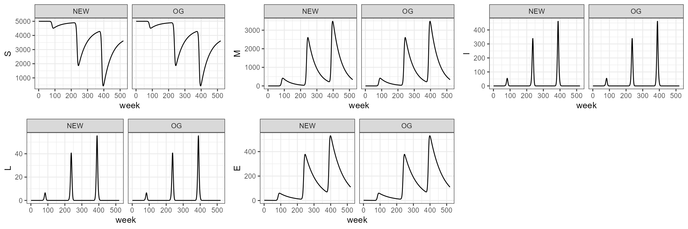
smile3
Only births with no seasonal infection probability
# In this function we introduce population dynamics only as births at the begining of the year
# determined by density dependent reproduction with a carrying capacity of 5000.

smile3  <-  function(b,theta,tau,years){

    # Fixed parameters
    alpha   <-  1/52
    zeta    <-  0.88
    gamma   <-  0.9868
    psi     <-  1

    n.weeks     <-  years*52 + 1
    S<- M<- I<- L<-E <-N<-lambda<- array(0,dim=c(n.weeks),dimnames=list(1:(n.weeks)))
    N[1]        <-  5000
    S[1]        <-  N[1]
    L[1]    <-  1; E[1] <-  L[1]*psi

    for(t in 2:n.weeks){

        tm1 <-  t-1
        lambda[tm1] <-  lambda.t(theta=theta,tau=tau,b=b,E=E[tm1])
        births.happen   <-  as.numeric(t%%52==0)
        rep.prob    <-  rho.n(N[tm1])

        S[t]    <-  (S[tm1]*(1-lambda[tm1])) + M[tm1]*1/52 + rep.prob*(N[tm1])*births.happen
        I[t]    <-  S[tm1]*lambda[tm1]
        M[t]    <-  I[tm1]*zeta + M[tm1]*(1-(1/52))
        L[t]    <-  I[tm1]*(1-zeta)
        E[t]    <-  psi*L[tm1] + E[tm1]*gamma
        N[t]    <-  S[t]+M[t]

    }


    results     <-  list(Suceptibles=S[-1]
                        ,Immune=M[-1]
                        ,Infected=I[-1]
                        ,LIZ=L[-1]
                        ,Environment=E[-1]
                        ,lambda=lambda[-1])

    return(results)
}
# Case 3: With births and no seasonal infection probability
tau=10
b=0.001

# Case 3.0: Low Dispersion. Mean dispersion effort is 0.1
theta=100
sim3.0  <-  smile3(b=b,tau=tau,theta=theta,years=10)
If we don’t consider seasonal forcing, then b0 and b1 are left as
null (the default) and we give the parameter b_fixed for fixed infection
probability. When the argument age_struc is not set to
FALSE, the function will use the default parameters of
K and rho_pop to estimate birth pulses every
year. These default parameters of carrying capacity and reproductive
rate can be changed easily by adding them to the function as
arguments.
sim3_1 <- smile_main(tau = tau, b_fixed = b, theta = theta, years = 10)
# sim3_1 <- smile_main(tau = 10, b_fixed = 0.001, theta = 100, years = 10)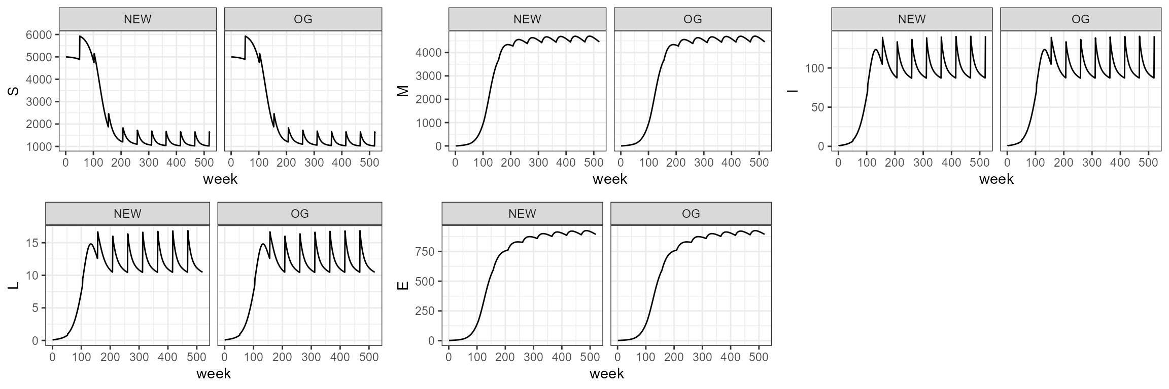
smile4
With births only and seasonal forcing of infection
# smile 4 function introduces population dynamics as in smile3 function but uses
# seasonal forcing for infection probability.

smile4  <-  function(b0,b1,period,theta,tau,years){

    # Fixed parameters
    alpha   <-  1/52
    zeta    <-  0.88
    gamma   <-  0.9868
    psi     <-  1

    n.weeks     <-  years*52 + 1
    S<- M<- I<- L<-E <-N<-lambda<- array(0,dim=c(n.weeks),dimnames=list(1:(n.weeks)))
    N[1]        <-  5000
    S[1]        <-  N[1]
    L[1]    <-  1; E[1] <-  L[1]*psi

    for(t in 2:n.weeks){

        tm1 <-  t-1
        b   <-  b.season(b0,b1,period,t)
        lambda[tm1] <-  lambda.t(theta=theta,tau=tau,b=b,E=E[tm1])
        births.happen   <-  as.numeric(t%%52==0)
        rep.prob    <-  rho.n(N[tm1])

        S[t]    <-  (S[tm1]*(1-lambda[tm1])) + M[tm1]*1/52 + rep.prob*(N[tm1])*births.happen
        I[t]    <-  S[tm1]*lambda[tm1]
        M[t]    <-  I[tm1]*zeta + M[tm1]*(1-(1/52))
        L[t]    <-  I[tm1]*(1-zeta)
        E[t]    <-  psi*L[tm1] + E[tm1]*gamma
        N[t]    <-  S[t]+M[t]

    }


    results     <-  list(Suceptibles=S[-1]
                        ,Immune=M[-1]
                        ,Infected=I[-1]
                        ,LIZ=L[-1]
                        ,Environment=E[-1]
                        ,lambda=lambda[-1])

    return(results)
}
tau=10
b0=-30
b1=0.85
period=3*52

# Case 4.0: Low Dispersion. Mean dispersion effort is 0.1
theta=100
sim4.0  <-  smile4(b0=b0,b1=b1,period=period,tau=tau,theta=theta,years=10)
In the function we change the parameter for deaths from non-disease
causes to sigmaa = 1, since the smile4 function does not
consider deaths from other causes. It is not necessary to change this
parameter though, since the default in the function is already set to
1.
sim4_1 <- smile_main(b0 = b0, b1 = b1, period = period, theta = theta, tau = tau, years = 10, sigmaa = 1)
# sim4_1 <- smile_main(b0 = -30, b1 = 0.85, period = 3*52, theta = 100, tau = 10, years = 10, sigmaa = 1)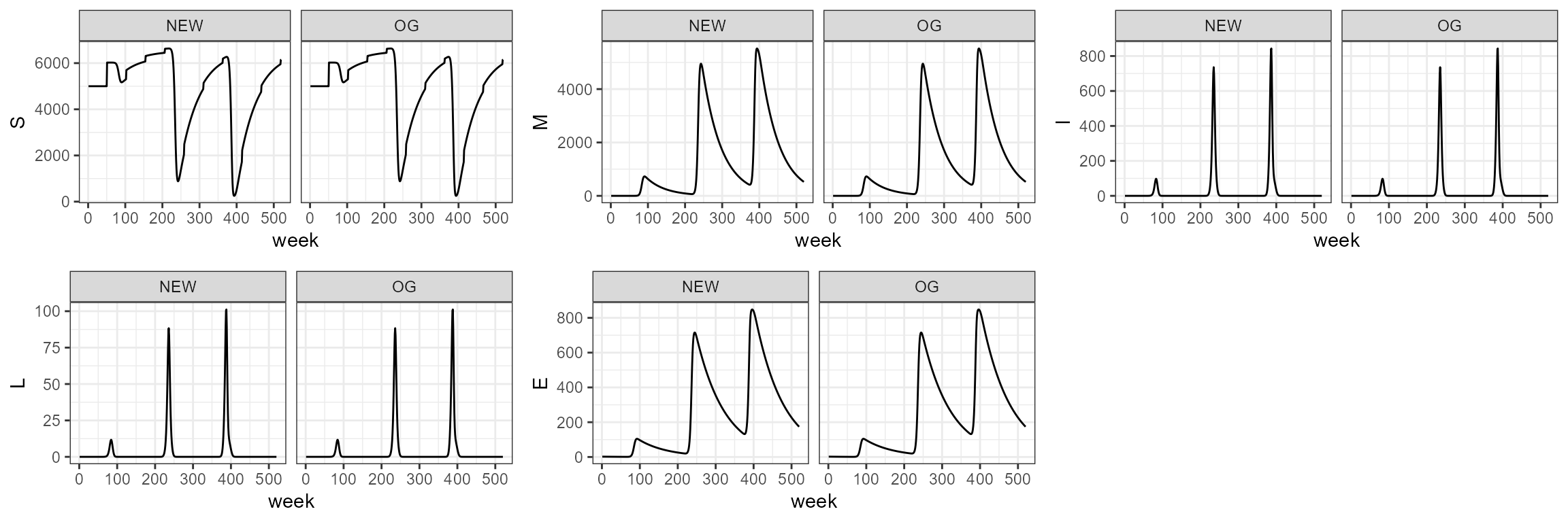
smile5
This one incorporates both host population dynamics and seasonal forcing, but additionally puts in the death by other causes.
# smile5 is the most realistic function of the group since it incorporates both births and deaths from other causes
# than the disease in population dynamics. Deaths are given by a 1- sigmaa = 1 - 0.92^(1/52)
smile5  <-  function(b0,b1,period,theta,tau,years){

    # Fixed parameters
    alpha   <-  1/52
    zeta    <-  0.88
    gamma   <-  0.9868
    sigmaa  <-  0.92^(1/52)
    psi     <-  1

    n.weeks     <-  years*52 + 1
    S<- M<- I<- L<-E <-N<-lambda<- array(0,dim=c(n.weeks),dimnames=list(1:(n.weeks)))
    N[1]        <-  5000
    S[1]        <-  N[1]
    L[1]    <-  1; E[1] <-  L[1]*psi

    for(t in 2:n.weeks){

        tm1 <-  t-1
        b   <-  b.season(b0,b1,period,t)
        lambda[tm1] <-  lambda.t(theta=theta,tau=tau,b=b,E=E[tm1])
        births.happen   <-  as.numeric(t%%52==0)
        rep.prob    <-  rho.n(N[tm1])

        S[t]    <-  (S[tm1]*(1-lambda[tm1]))*sigmaa + M[tm1]*sigmaa*1/52 + rep.prob*(N[tm1])*births.happen
        I[t]    <-  S[tm1]*lambda[tm1]
        M[t]    <-  I[tm1]*zeta + M[tm1]*sigmaa*(1-(1/52))
        L[t]    <-  I[tm1]*(1-zeta)
        E[t]    <-  psi*L[tm1] + E[tm1]*gamma
        N[t]    <-  S[t]+M[t]

    }


    results     <-  list(Suceptibles=S[-1]
                        ,Immune=M[-1]
                        ,Infected=I[-1]
                        ,LIZ=L[-1]
                        ,Environment=E[-1])

    return(results)
}
tau=10
b0=-30
b1=0.85
period=3*52

# Case 5.0: Low Dispersion. Mean dispersion effort is 0.1
theta=10
sim5.0      <-  smile5(b0=b0,b1=b1,period=period,tau=tau,theta=theta,years=10)
sim5_1 <- smile_main(b0 = b0, b1 = b1, period = period, theta = theta, tau = tau, years = 10, sigmaa = 0.92^(1/52))
# sim5_1 <- smile_main(b0 = -30, b1 = 0.85, period = 3*52, theta = 10, tau = 10, years = 10, sigmaa = 0.92^(1/52))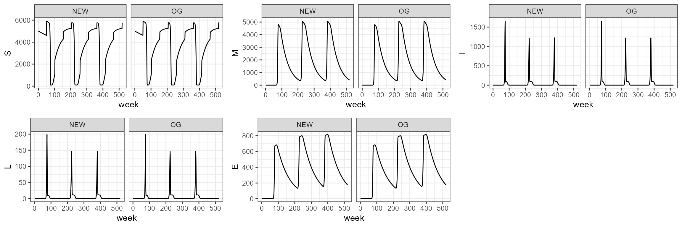
Stochastic version of the last one:
# Final function is the stochastic version of smile5 function. It incorporates births, deaths by disease
# and other causes and seasonal forcing of the infection probability. The stochasticity is introduced by
# assuming that Infected, Immune and LIZ are all binomial random variables. I allowed stochasticity in the
# number of spores introduced to the environment by assuming that it is poisson random variable with mean
# given by the number of diseas deaths times a constant. Virulence of spores that remain virulent in the
# environment is also a binomial random variable with with probability of succes gamma = 0.9868.

smile5.stoch    <-  function(b0,b1,period,theta,tau,years){

    # Fixed parameters
    alpha   <-  1/52
    zeta    <-  0.88
    gamma   <-  0.9868
    sigmaa  <-  0.92^(1/52)
    psi     <-  1

    n.weeks     <-  years*52 + 1
    S<- M<- I<- L<-E <-N<-lambda<- array(0,dim=c(n.weeks),dimnames=list(1:(n.weeks)))
    N[1]        <-  5000
    S[1]        <-  N[1]
    L[1]    <-  1; E[1] <-  rpois(1,L[1]*psi    )

    for(t in 2:n.weeks){

        tm1 <-  t-1
        b   <-  b.season(b0,b1,period,t)
        lambda[tm1] <-  lambda.t(theta=theta,tau=tau,b=b,E=E[tm1])
        births.happen   <-  as.numeric(t%%52==0)
        rep.prob    <-  rho.n(N[tm1])

        I[t]    <-  rbinom(1,S[tm1],lambda[tm1])
        births  <-  rbinom(1,N[tm1],rep.prob)*births.happen
        M.surv  <-  rbinom(1,M[tm1],sigmaa)
        M.recov <-  rbinom(1,M.surv,alpha)
        M.new   <-  rbinom(1,I[tm1],zeta)
        S[t]    <-  rbinom(1,S[tm1]-I[t],sigmaa) + M.recov + births
        M[t]    <-  M.new + (M.surv - M.recov)
        L[t]    <-  (I[tm1]-M.new)
        E[t]    <-  rpois(1,psi*L[tm1]) + rbinom(1,E[tm1],gamma)
        N[t]    <-  S[t]+M[t]

    }


    results     <-  list(Suceptibles=S[-1]
                        ,Immune=M[-1]
                        ,Infected=I[-1]
                        ,LIZ=L[-1]
                        ,Environment=E[-1])

    return(results)
}
stochastic.sims <-  list()
LIZ.stoch       <-  matrix(0,nrow=100,ncol=520)
for(i in 1:100){

    stochastic.sims[[i]]    <-  smile5.stoch(b0=b0,b1=b1,period=period,tau=tau,theta=theta,years=10)
    LIZ.stoch[i,]           <-  stochastic.sims[[i]]$LIZ

}
stochastic_sims <-  list()
LIZ_stoch       <-  matrix(0,nrow=100,ncol=520)
for(i in 1:100){

    stochastic_sims[[i]]    <-  smile_main(b0 = b0, b1 = b1, period = period, theta = theta, tau = tau, years = 10, sigmaa = 0.92^(1/52),
                                       stochastic = TRUE)
    LIZ_stoch[i,]           <-  stochastic_sims[[i]]$LIZ

}
as.data.frame(LIZ.stoch) %>% rownames_to_column(var = "sim") %>%
  pivot_longer(-sim, names_to = "week", values_to = "n_LIZ") %>%
  mutate(week = str_remove(week, "V"), week = as.numeric(week)) %>%
  mutate(model = "OG") -> og_stochastic

as.data.frame(LIZ_stoch) %>% rownames_to_column(var = "sim") %>%
  pivot_longer(-sim, names_to = "week", values_to = "n_LIZ") %>%
  mutate(week = str_remove(week, "V"), week = as.numeric(week)) %>%
  mutate(model = "NEW") -> new_stochastic
Very similar results, considering this is the stochastic versions. It makes sense.
bind_rows(og_stochastic, new_stochastic) %>%
  # filter(sim %in% 10:15) %>%
  ggplot(aes(x = week, y = n_LIZ, group = sim)) +
  facet_wrap(~model) +
  # facet_grid(sim~model) +
  geom_line() +
  theme_minimal()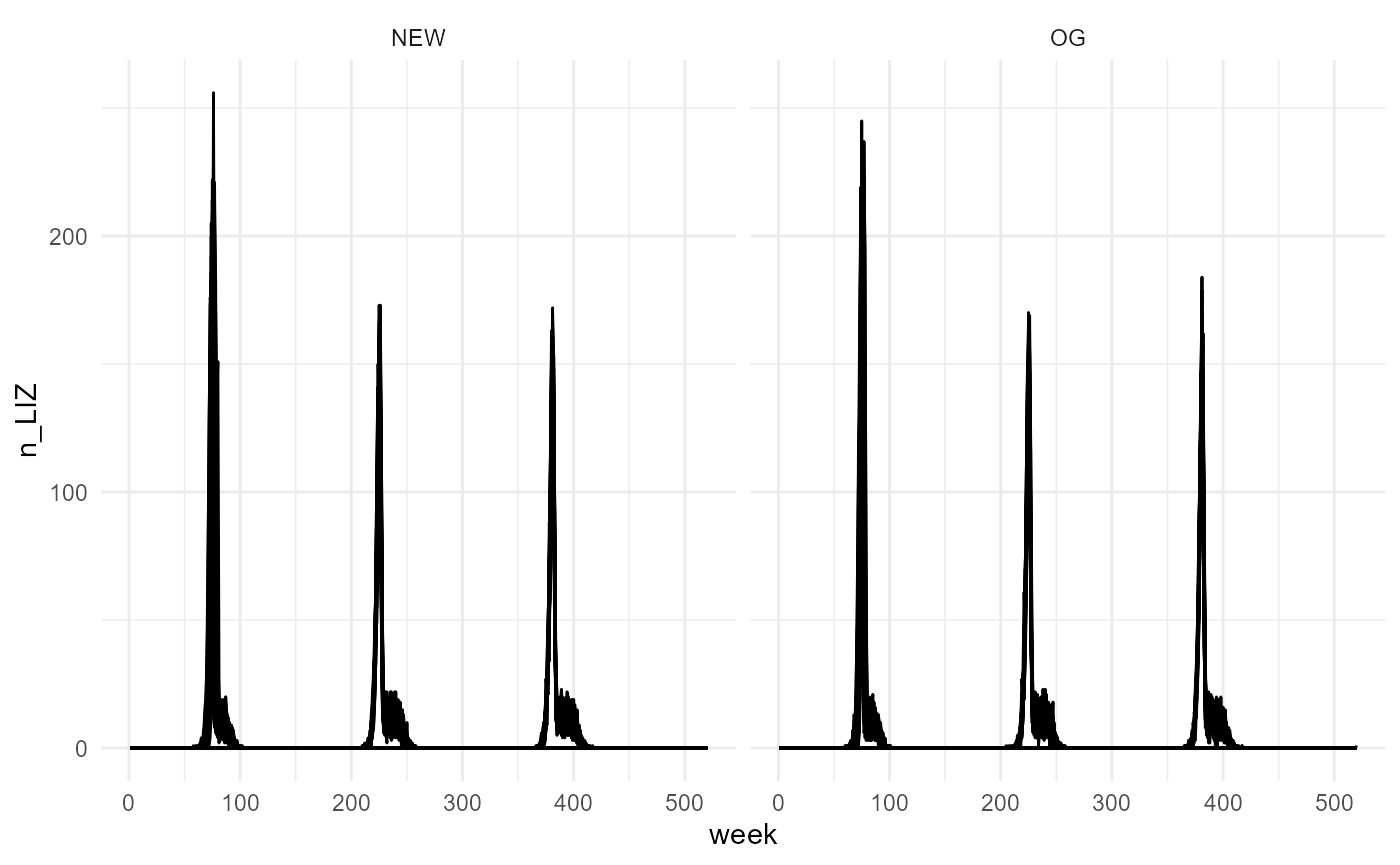
Estimation
Estimation of parameters using the last scenario and stochastic simulations
# Functions for estimating the parameters of the SMILE model b0, b1, period, theta and tau.
# The estimation assumes that the observed LIZ are poisson distributed product of observation error
# and not process error as properly described in the smile5.stoch function. This is a set of two functions
# the first one gives the negative loglikelihood of the model that will be minimized using the optim function.
# The second one is a wrapper of the optim function that returns the maximum likelihood estimates of the parameters.
# Period must be in weeks and SMILE.obs must follow exactly the formating of the output of one of the above SMILE
# functions.

LIZ.negll   <-  function(pars=c(theta,tau,b0,b1),period,years,SMILE.obs){

    theta   <-  exp(pars[1])
    tau     <-  exp(pars[2])
    b0      <-  pars[3]
    b1      <-  pars[4]
    # Likelihood of infection seasonality as a function of climate

    #wt.bar.hat <-  mean(clim)
    #clim.pred  <-  infect2clim(wt.bar=wt.bar.hat,b0=b0,b1=b1,kw=kw,t=1:length(clim),period=period)
    #clim.ssq   <-  sum((clim-clim.pred)^2)

    SMILE.pred  <-  smile5(b0,b1,period,theta,tau,years)
    ts2keep     <-  names(SMILE.pred)%in%names(SMILE.obs)
    SMILE.pred  <-  SMILE.pred[which(ts2keep==TRUE)]
    loglik.ls   <-  vector("list",length(SMILE.obs))

    for(i in 1:length(SMILE.obs)){

        loglik.ls[[i]]  <-  dpois(SMILE.obs[[i]],SMILE.pred[[i]],log=TRUE)

    }

    loglik.ls   <-  lapply(loglik.ls,sum)

    loglik  <-  sum(unlist(loglik.ls))

    if(!is.finite(loglik)){loglik=-.Machine$double.xmax}
    negll   <-  -loglik #+ clim.ssq
    return(negll)

}

SMILE.param.estim   <-  function(b0,b1,theta,tau,period,SMILE.obs,method="BFGS"){

    years       <-  length(SMILE.obs[[1]])/52
    pars        <-  c(theta,tau,b0,b1)

    optim.res   <-  optim(par=pars,fn=LIZ.negll,method=method,SMILE.obs=SMILE.obs
                                ,years=years,period=period)

    theta.hat   <-  exp(optim.res$par[1])
    tau.hat     <-  exp(optim.res$par[2])
    b0.hat      <-  optim.res$par[3]
    b1.hat      <-  optim.res$par[4]


    neg.ll      <-  optim.res$value

    results     <-  c(tau=tau.hat,theta=theta.hat,b0=b0.hat,b1=b1.hat,loglik=-neg.ll)
    return(results)
}
set.seed(123)
b0_start    <-  runif(1,min=-36,max=-24)
b1_start    <-  runif(1,min=0.656,max=0.984)
theta_start <-  log(runif(1,min=8,max=12))
tau_start   <-  log(runif(1,min=8,max=12))

SMILE_obs <- stochastic.sims
nreps <- length(SMILE_obs)

hat_mat         <-  array(0,dim=c(nreps,5),dimnames=list(1:nreps
                                                             ,c("tau","theta","b0","b1","loglik")))

for(i in 1:nreps){

    hat_mat[i,] <-  SMILE.param.estim(b0 = b0_start,
                                     b1 = b1_start,
                                     theta = theta_start,
                                     tau = tau_start,
                                     SMILE.obs=SMILE_obs[[i]],period=3*52)
                                }
with the new functions
set.seed(123)
b0_start    <-  runif(1,min=-36,max=-24)
b1_start    <-  runif(1,min=0.656,max=0.984)
theta_start <-  log(runif(1,min=8,max=12))
tau_start   <-  log(runif(1,min=8,max=12))

SMILE_obs <- stochastic_sims
nreps <- length(SMILE_obs)

hat_mat         <-  array(0,dim=c(nreps,5),dimnames=list(1:nreps
                                                             ,c("tau","theta","b0","b1","loglik")))

for(i in 1:nreps){

    hat_mat[i,] <-  SMILE_param_estim(b0 = b0_start,
                                     b1 = b1_start,
                                     theta = theta_start,
                                     tau = tau_start,
                                     SMILE.obs=SMILE_obs[[i]],period=3*52)
                                }
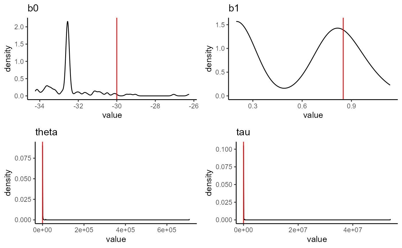
Parameter estimates for each of the stochastic simulations we generated. All simulations used the values shown with the red line to be generated.
